Tutorial: LDBC Gremlin
Prior to beginning, it is important to note that LDBC is a highly regarded organization in the realm of graph databases/systems benchmark standards and audit testing. LDBC has developed several benchmark toolsuits, with GIE primarily focusing on the Social Network Benchmark (SNB). This benchmark defines graph workloads specifically for database management systems, including both interactive (high-QPS) workloads and business intelligence workloads.
During this tutorial, we will walk you through various use cases when querying the simulated social network utilized in SNB. By the conclusion of this tutorial, we are confident that you will be proficient in constructing Gremlin queries that are just as intricate as the business intelligence workloads found in SNB.
Load the LDBC Graph
For this tutorial, we will use the LDBC social network as the graph data, which has the following entities:
vertex/edge labels(types) in the graph
connections and relationships among labels
properties related all kinds of labels
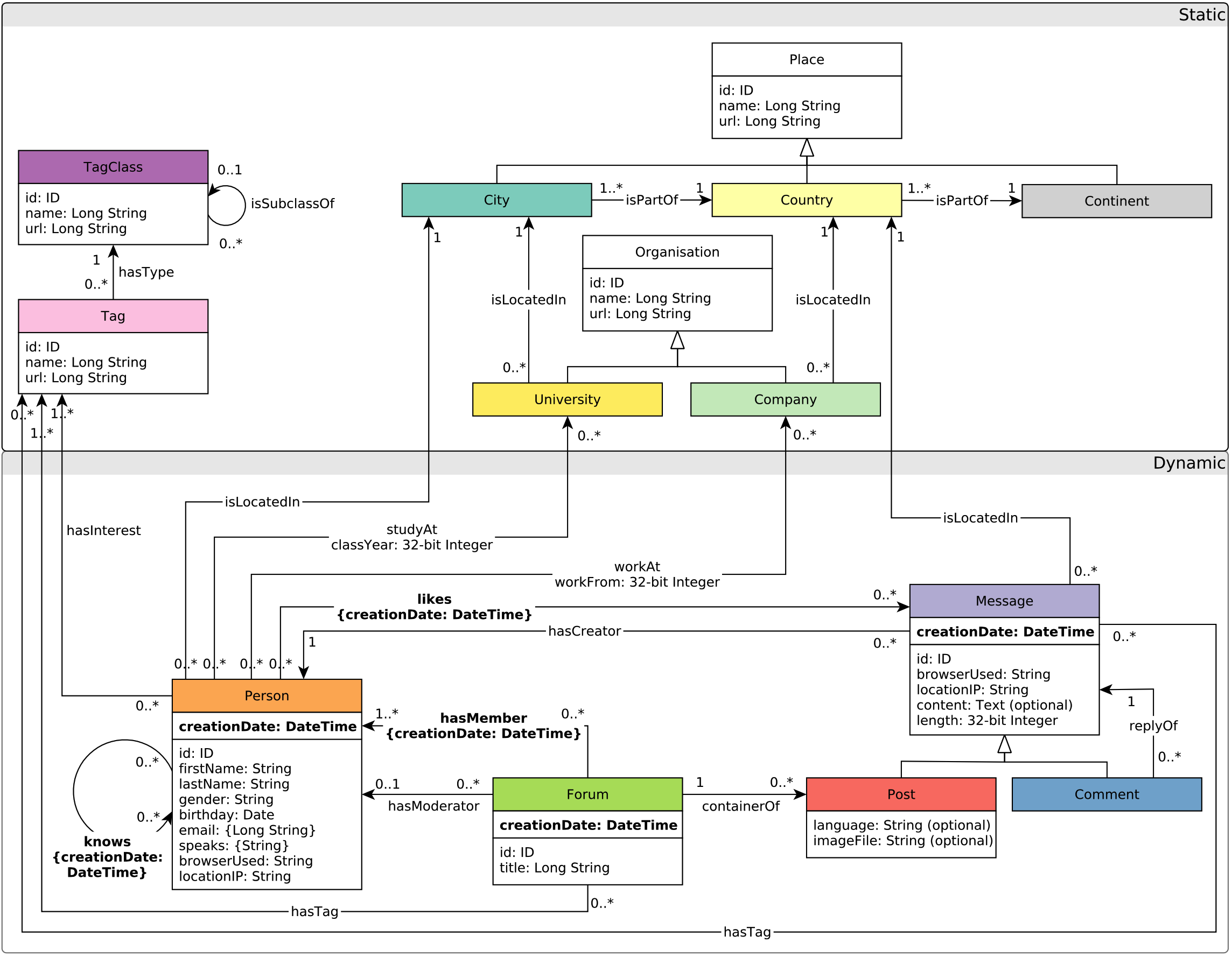
Figure 1. The schema of the LDBC graph (referred to LDBC SNB).
LDBC graph is one of the built-in dataset of GraphScope, so it can be easily loaded through:
from graphscope.dataset.ldbc import load_ldbc

graph = load_ldbc()
This will load the LDBC social network with the scale factor (sf) 1.
Tip
We do permit loading much larger LDBC graphs, such as sf 3k. To handle such large graphs, you’re recommended using the standalone deployment of GIE in a large cluster.
Currently, GIE supports Gremlin as its query language.
After loading the LDBC graph and initializing the engine, we can submit Gremlin queries to GIE through g.execute(GREMLIN_QUERIES) easily.
For example, if we want to count there are how many vertices and edges in the LDBC graph, we can simply write the following python codes:
import graphscope as gs
from graphscope.dataset.ldbc import load_ldbc

# load the ldbc graph
graph = load_ldbc()

# Hereafter, you can use the `graph` object to create an `gremlin` query session
g = gs.gremlin(graph)
# then `execute` any supported gremlin query.
# count vertices
q1 = g.execute('g.V().count()')
print(q1.all().result())
# count edges
q2 = g.execute('g.E().count()')
print(q2.all().result())
Then the output should be:
[190376]
[787074]
It suggests that there are 190376 vertices and 787074 edges in the LDBC sf1 graph.
Basic Vertex/Edge Query
It is very common to use SQL sentences to retrieve data from relational databases. In graph, vertices can be regarded as entities, and edges can be regarded as the connecting relationship among entities. Similarly, we can easily retrieve data from graph with GIE and corresponding graph query sentences.
Retrieve Vertices and Edges
As shown in the last tutorial, we can easily retrieve vertices and edges from graph through g.V() and g.E() Gremlin steps.
# then `execute` any supported gremlin query.
# Retrieve all vertices
q1 = g.execute('g.V()')
print(q1.all().result())
# Retrieve all edges
q2 = g.execute('g.E()')
print(q2.all().result())
The output of the above code should be like:
# All vertices
[v[432345564227583365], ......, v[504403158265495622]]
# All edges
[e[576460752303435306][432345564227579434-hasType->504403158265495612], ......, e[144115188075855941][504403158265495622-isSubclassOf->504403158265495553]]
For vertices, the number inside [] represents its id. However, the ids seem to be a little bit confusing: why are they so large? Actually, such large ids result from the different storage mechanism between graph and relational databases.
In relational databases, instances with different types are stored separately in different tables. Therefore, we usually use local id to retrieve specific instance from the table. For example, we can use select * from Person where id=0 to retrieve person with id=0 from the Person table. Since the id is local, instances belonging to different tables may have the same id (e.g. person(id=0) and message(id=0)).
When it comes to graph storage, all kinds of vertices and edges are stored together. If it still uses local id to locate vertices and edges, there will be many conflicts. Therefore, every vertex and edge needs a specific global identifier, called global id, to distinguish it from others.
GIE uses global id to identify very vertex and edge. The ids look so large mainly because the underlying storage generates vertex’s global id from its local id and label by some bit operations(shift and plus). After all, the global ids are just identifiers, and we don’t need to worry too much about what it looks like.
For edges, still the number inside the first [] represents its id. The content inside the second [] is of the format source vertex id -edge label(type)-> destination vertex id,indicating the edge’s two end vertices’ id and the connection type (edge label).
Apply Some Filters
In most cases, we don’t need to retrieve all the vertices and edges from the graph, as we may only care about a small portion of them. Therefore, GIE with Gremlin provides you with some filtering operations to help find the data you are interested in.
If you only want to extract a vertex/edge with the given id, you can write Gremlin sentence g.V(id) in GIE. (g.E(id) will be supported in the future)
# Retrieve vertex with id 1
q1 = g.execute('g.V(1)')
print(q1.all().result())
The output should be like:
[v[1]]
Sometimes, you may want to retrieve vertices/edges having a specific label, you can use haveLabel(label) step in Gremlin. For example, the following codes show how to find all person vertices.
# Retrieve vertices having label 'person'
q1 = g.execute('g.V().hasLabel("person")')
print(q1.all().result())
The output should be like:
# All person vertices
[v[216172782113783808], ......, v[216172782113784710]]
If you want to extract more than one type(label) of vertices, you can write many labels in the step, like haveLabel(label1, label2...). For example, the following codes extracts all the vertices having label ‘person’ or ‘forum’.
# Retrieve vertices having label 'person' or 'forum'
q1 = g.execute('g.V().hasLabel("person", "forum")')
print(q1.all().result())
The output should be like:
# All person vertices and forum vertices
[v[216172782113783808], ......,  v[72057594037936036]]
As mentioned in the last tutorial, GraphScope models data graph as property graph, so GIE allows user to filter the outputs according to some properties by using has(...) step.
The usage of has(...) step is very flexible. Firstly, it allows user to find vertices having some required properties. For example, the following codes aims to extract vertices having property ‘creationDate’
# Retrieve vertices having property 'creationDate'
q1 = g.execute('g.V().has("creationDate")')
print(q1.all().result())
The output should be like:
# All vertices having property 'creationDate'
v[360287970189718653], ......, v[360287970189718655]]
From the LDBC schema shown above, you can see that vertices with label ‘person’, ‘forum’, ‘post’ and ‘comment’ all have property ‘creationDate’. Therefore, the above query sentence is equivalent to:
# Retrieve vertices having label 'person' or 'forum' or 'message'
q1 = g.execute('g.V().hasLabel("person", "forum", "comment", "post")')
print(q1.all().result())
In addition, you may further require the extracted properties satisfying some conditions. For example, if you want to extract persons whose first name is ‘Joseph’, you can write the following codes:
# Retrieve person vertices whose first name is 'Joseph'
q1 = g.execute('g.V().hasLabel("person").has("firstName", "Joseph")')
print(q1.all().result())
You can also write more complicated predicates in the has(...) step, for example:
# Retrieve person vertices whose first name is not 'Joseph'
q1 = g.execute('g.V().hasLabel("person").has("firstName", not(eq("Joseph")))')
# Retrieve person vertices whose first name is either 'Joseph' or 'Yacine'
q2 = g.execute('g.V().hasLabel("person").has("firstName", within("Joseph", "Yacine"))')
# Retrieve comment vertices created after the very beginning of year 2011
q3 = g.execute('g.V().hasLabel("comment").has("creationDate", gt( "2011-01-01T00:00:00.000+0000"))')
print(q1.all().result())
print(q2.all().result())
print(q3.all().result())
Here are more references about has(...) step in Gremlin.
Extract Property Values
Sometimes, you may more curious about the property values of the vertices/edges. With GIE, you can easily use values(PROPERTY_NAME) Gremlin step to extract the vertices/edges’ property value.
For example, you have already known that vertex(id=38416) is a comment, and you are interested in its content, then you can write the following codes in GIE:
# Extract comment vertex(id=38416)'s content
q1 = g.execute('g.V(38416).values("content")')
print(q1.all().result())
The output should be like:
# The content of the comment(id=38416)
['maybe']
Real Applications
Since GIE provides python interface, it is very convenient to do some further data analytics on the retrieved data.
Here is an example about the statistics of the comment content’s length (word count) in the LDBC Graph.
import matplotlib.pyplot as plt
import graphscope as gs
from graphscope.dataset.ldbc import load_ldbc

# load the modern graph as example.
graph = load_ldbc()

# Hereafter, you can use the `graph` object to create an `gremlin` query session
g = gs.gremlin(graph)

# Extract all comments' contents
q1 = g.execute('g.V().hasLabel("comment").values("content")')
comment_contents = q1.all().result()
comment_length = [len(comment_content.split()) for comment_content in comment_contents];

# Draw Histogram
plt.hist(x=list(filter(lambda x:(x< 50), comment_length)), bins='auto', color='#607c8e',alpha=0.75)
plt.grid(axis='y', alpha=0.75)
plt.xlabel('Comments Length')
plt.ylabel('Comments Count')
plt.title('Comment Length Histogram')
plt.show()
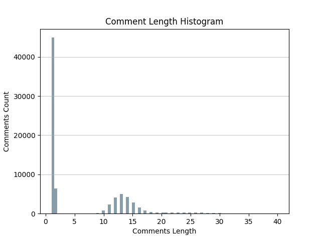
Figure 2. The histogram of the comments’ length in the ldbc social network.
We can also draw a pie chart about the gender ratio in the social network.
import matplotlib.pyplot as plt
import graphscope as gs
from graphscope.dataset.ldbc import load_ldbc


# load the modern graph as example.
graph = load_ldbc()

# Hereafter, you can use the `graph` object to create an `gremlin` query session
g = gs.gremlin(graph)

# Extract all person' gender property value
q1 = g.execute('g.V().hasLabel("person").values("gender")')
person_genders = q1.all().result()
# Count male and female
male_count = 0
female_count = 0
for gender in person_genders:
    if gender == "male":
        male_count += 1
    else:
        female_count += 1

# Draw pie chart
plt.pie(x=[male_count, female_count], labels=["Male", "Female"])
plt.show()
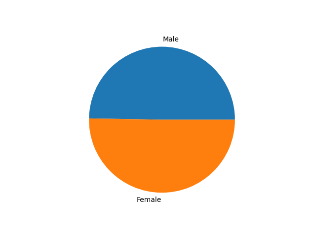
Figure 3. The pie chart of person’s gender in the ldbc social network.
Basic Traversal Query
The main difference between Property Graph and Relational Database is that Property Graph treats the relationship(edges) among entities(vertices) at the first class. Therefore, it is easy to walk through vertices and edges in the Property Graph according to some pre-defined paths.
In GIE, we call such walk as Graph Traversal: This type of workload involves traversing the graph from a set of source vertices while satisfying the constraints on the vertices and edges that the traversal passes. Graph traversal differs from the analytics workload as it typically accesses a small portion of the graph rather than the whole graph.
In this tutorial, we would like to discuss how to use Gremlin steps to traverse the Property Graph. Furthermore, we will show some examples about how to apply graph traversals in real world data analytics.
Expansion
The most basic unit in Graph Traversal is Expansion, which means starting from a vertex/edge and reaching its adjacencies. GIE currently supports the following expansion steps in Gremlin:
out(): Map the vertex to its outgoing adjacent vertices given the edge labels.in(): Map the vertex to its incoming adjacent vertices given the edge labels.both(): Map the vertex to its adjacent vertices given the edge labels.outE(): Map the vertex to its outgoing incident edges given the edge labels.inE(): Map the vertex to its incoming incident edges given the edge labels.bothE(): Map the vertex to its incident edges given the edge labels.outV(): Map the edge to its outgoing/tail incident vertex.inV(): Map the edge to its incoming/head incident vertex.otherV(): Map the edge to the incident vertex that was not just traversed from in the path history.bothV():Map the edge to its incident vertices.
Here is a local subgraph extracted from the LDBC Graph, which is formed by a center person vertex (id=216172782113784483) and all of its adjacent edges and vertices. Then we will use this subgraph to explain all of the expansion steps.
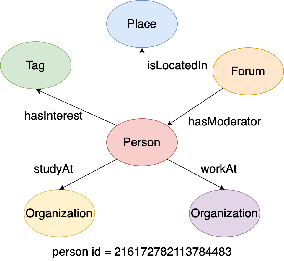
Figure 5. A local graph around a given person vertex.
out(), in() and both()
All of these three steps start traverse from source vertices to their adjacent vertices. The differences between them are:
out()traverse through the outgoing edges to the adjacent verticesin()traverse through the incoming edges to the adjacent verticesboth()traverse through both of the outgoing and incoming edges to the adjacent vertices
For example, if you want to find vertex(id=216172782113784483)’s adjacent vertices by the three steps, you can write sentences in GIE like:
# Traverse from the vertex to its adjacent vertices through its outgoing edges
q1 = g.execute('g.V(216172782113784483).out()')
# Traverse from the vertex to its adjacent vertices through its incoming edges
q2 = g.execute('g.V(216172782113784483).in()')
# Traverse from the vertex to its adjacent vertices through all of its incident edges
q3 = g.execute('g.V(216172782113784483).both()')
print(q1.all().result())
print(q2.all().result())
print(q3.all().result())
This figure illustrates the execution process of q1, q2 and q3:
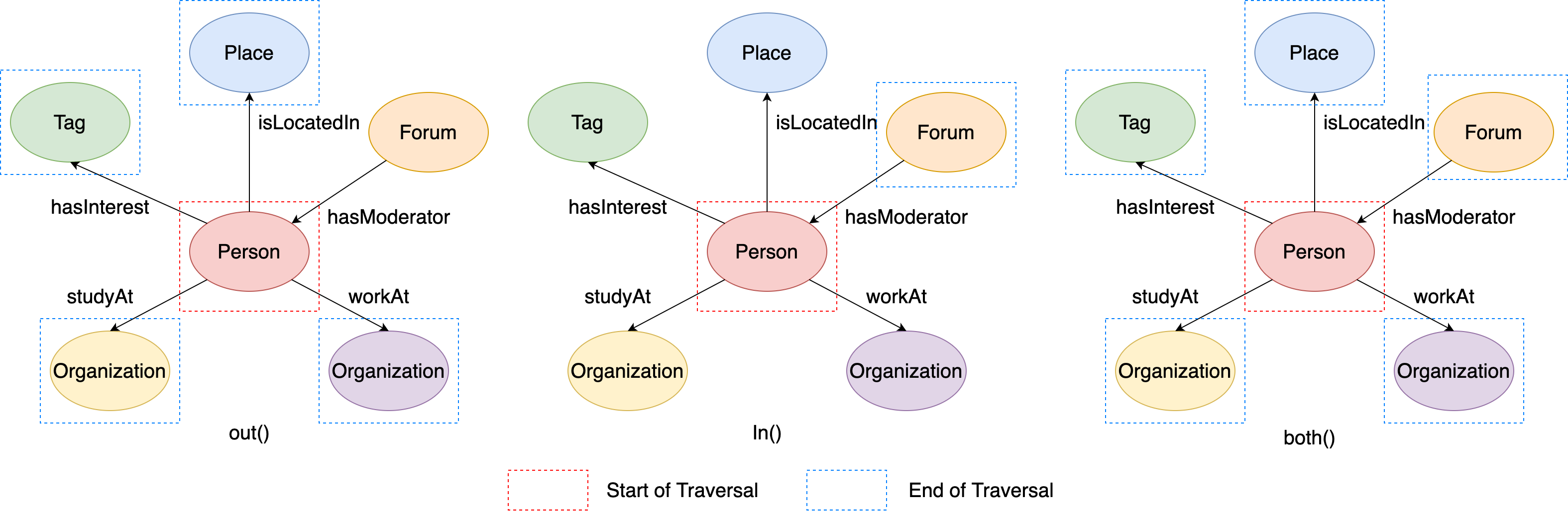
Figure 6. The examples of out/in/both steps.
Therefore, the output of the above codes should be like:
# q1: vertex's adjacent vertices through outgoing edges
[v[432345564227569033], v[288230376151712472], v[144115188075856168], v[144115188075860911]]
# q2: vertex's adjacent vertices through incoming edges
[v[72057594037934114]]
# q3: vertex's adjacent vertices through all of its incident edges
[v[432345564227569033], v[288230376151712472], v[144115188075856168], v[144115188075860911], v[72057594037934114]]
In addition, the three steps all support using edge labels as its parameters to further limit the traversal edges, like out/in/both(label1, label2, ...), which means it only can traverse through the edges whose label is one of {label 1, label 2, …, label n}. For example:
# Traverse from the vertex to its adjacent vertices through its incoming edges, and the edge label should be 'hasModerator'
q1 = g.execute('g.V(216172782113784483).in("hasModerator")')
# Traverse from the vertex to its adjacent vertices through its outgoing edges, and the edge label should be either 'studyAt' or 'workAt'
q2 = g.execute('g.V(216172782113784483).out("studyAt", "workAt")')
# Traverse from the vertex to its adjacent vertices through all of its incident edges, and the edge label should be either 'isLocatedIn' or 'hasModerator'
q3 = g.execute('g.V(216172782113784483).both("isLocatedIn", "hasModerator")')
print(q1.all().result())
print(q2.all().result())
print(q3.all().result())
This figure illustrates the execution process of q1, q2 and q3:
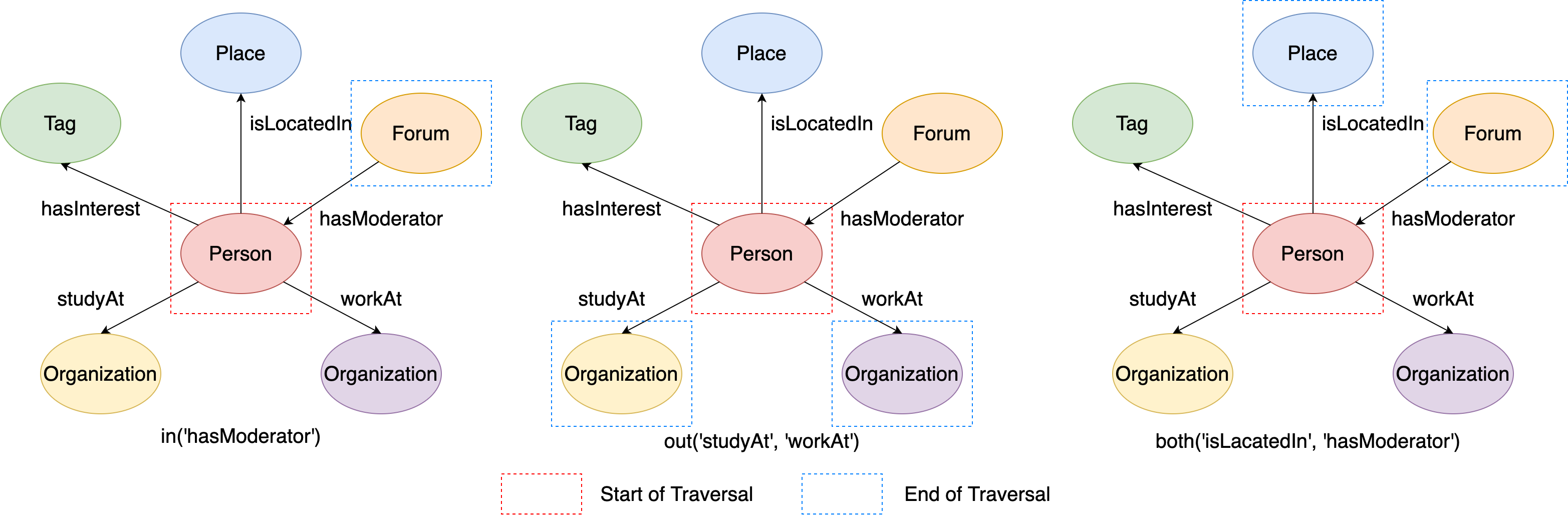
Figure 7. The examples of out/in/both steps from given labels.
Therefore, the output of the above codes should be like:
# q1: vertex's adjacent vertices through incoming 'hasModerator' edges
[v[72057594037934114]]
# q1: vertex's adjacent vertices through outgoing 'studyAt' or 'workAt' edges
[v[144115188075860911], v[144115188075856168]]
# q1: vertex's adjacent vertices through 'isLocatedIn' or 'hasModerator' edges
[v[288230376151712472], v[72057594037934114]]
outE(), inE() and bothE()
All of these three steps start traverse from source vertices to their adjacent edges. Similar to out(), in() and both(), the differences between them are:
outE()can only traverse to the outgoing adjacent edges of the source verticesinE()can only traverse to the incoming adjacent edges of the source verticesbothE()can traverse to both of the outgoing and incoming adjacent edges of the source vertices
For example, if you want to find vertex(id=216172782113784483)’s adjacent edges by the three steps, you can write sentences in GIE like:
# Traverse from the vertex to its outgoing adjacent edges
q1 = g.execute('g.V(216172782113784483).outE()')
# Traverse from the vertex to its incoming adjacent edges
q2 = g.execute('g.V(216172782113784483).inE()')
# Traverse from the vertex to all of its adjacent edges
q3 = g.execute('g.V(216172782113784483).bothE()')
print(q1.all().result())
print(q2.all().result())
print(q3.all().result())
This figure illustrates the execution process of q1, q2 and q3:
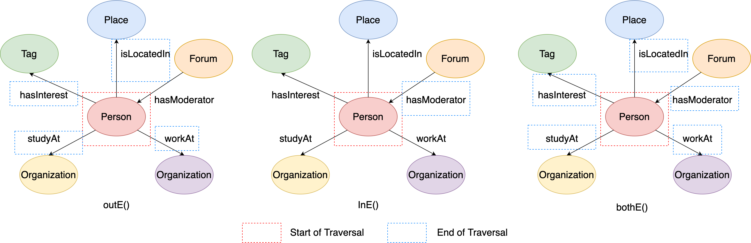
Figure 8. The examples of outE/inE/bothE steps.
Therefore, the output of the above codes should be like:
# q1: vertex's incident outgoing edges
[e[432345564227582847][216172782113784483-hasInterest->432345564227569033], e[504403158265496227][216172782113784483-isLocatedIn->288230376151712472], e[864691128455136658][216172782113784483-workAt->144115188075856168], e[1008806316530991636][216172782113784483-studyAt->144115188075860911]]
# q2: vertex's incident incoming edges
[e[360287970189645858][72057594037934114-hasModerator->216172782113784483]]
# q3: vertex's incident edges
[e[360287970189645858][72057594037934114-hasModerator->216172782113784483], e[432345564227582847][216172782113784483-hasInterest->432345564227569033], e[504403158265496227][216172782113784483-isLocatedIn->288230376151712472], e[864691128455136658][216172782113784483-workAt->144115188075856168], e[1008806316530991636][216172782113784483-studyAt->144115188075860911]]
Similarly, the three steps also support using edge labels as its parameters to further limit the traversal edges, like outE/inE.bothE(label1, label2, ...), which means it only can traverse to the edges whose label is one of {label 1, label 2, …, label n}. For example:
# Traverse from the vertex to its incident incoming edges, and the edge label should be 'hasModerator'
q1 = g.execute('g.V(216172782113784483).inE("hasModerator")')
# Traverse from the vertex to its incident outgoing edges, and the edge label should be either 'studyAt' or 'workAt'
q2 = g.execute('g.V(216172782113784483).outE("studyAt", "workAt")')
# Traverse from the vertex to its incident edges, and the edge label should be either 'isLocatedIn' or 'hasModerator'
q3 = g.execute('g.V(216172782113784483).bothE("isLocatedIn", "hasModerator")')
print(q1.all().result())
print(q2.all().result())
print(q3.all().result())
This figure illustrates the execution process of q1, q2 and q3:
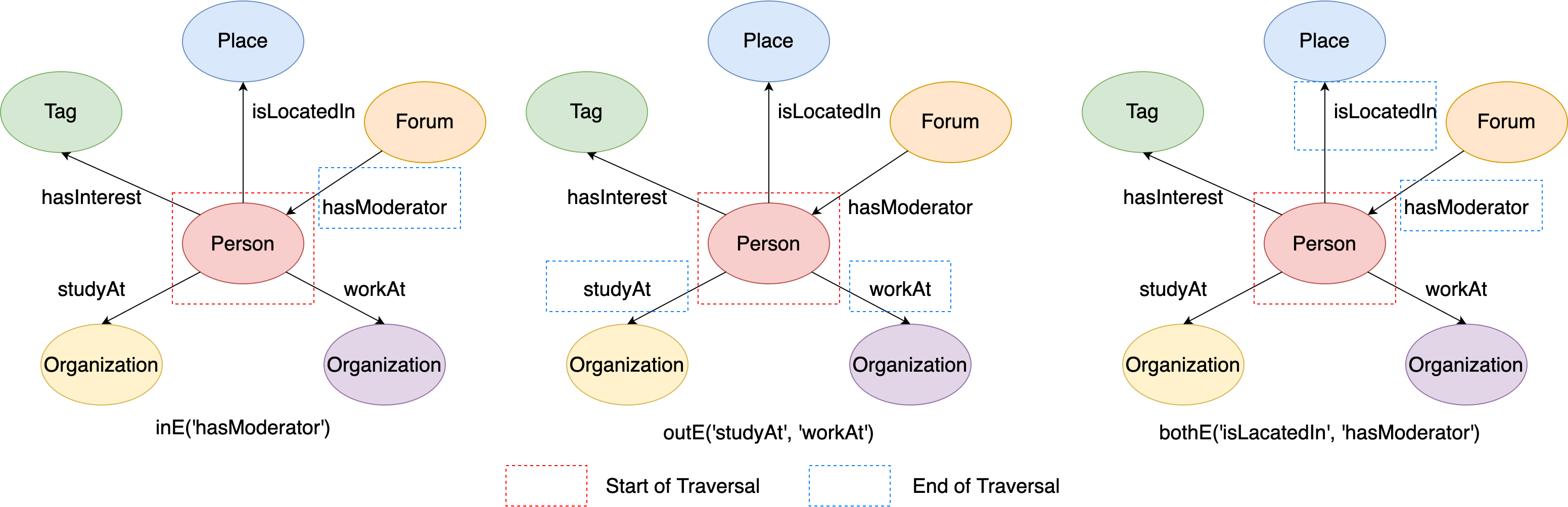
Figure 9. The examples of outE/inE/bothE steps from given labels.
Therefore, the output of the above codes should like:
# q1: vertex's incident incoming 'hasModerator' edges
[e[360287970189645858][72057594037934114-hasModerator->216172782113784483]]
# q2: vertex's incident outgoing 'studyAt' or 'workAt' edges
[e[1008806316530991636][216172782113784483-studyAt->144115188075860911], e[864691128455136658][216172782113784483-workAt->144115188075856168]]
# q3: vertex's incident 'isLocatedIn' or 'hasModerator' edges
[e[360287970189645858][72057594037934114-hasModerator->216172782113784483], e[504403158265496227][216172782113784483-isLocatedIn->288230376151712472]]
outV(), inV(), bothV() and otherV()
When reaching an edge during the traversal, you may be interested in its incident vertices. Therefore, GIE supports Gremlin steps that traverse from source edges to their incident vertices.
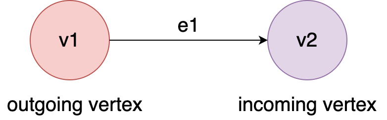
Figure 10. The examples of outgoing/incoming vertex of an edge.
For en edge e1 whose direction is from v1 to v2, we call v1 as ‘outgoing vertex’ and v2 as ‘incoming’ vertices.
outV(): traverse from source edges to the outgoing verticesinV(): traverse from source edges to the incoming verticesbothV(): traverse from source edges to both of the outgoing and incoming verticesotherV(): this step is a little bit special, it traverse from source edges to the incident vertices that haven’t appear in the traversal history. It will be explained in details later.
In the local subgraph, assume that currently we are at ‘isLocatedIn’ edge. If you want to get its incident vertices through outV()/inV()/bothV() step, you can write sentences in GIE like:
# Traverse from the edge to its outgoing incident vertex
q1 = g.execute('g.V(216172782113784483).outE("isLocatedIn").outV()')
# Traverse from the edge to its incoming incident vertex
q2 = g.execute('g.V(216172782113784483).outE("isLocatedIn").inV()')
# Traverse from the edge to both of its incident vertex
q3 = g.execute('g.V(216172782113784483).outE("isLocatedIn").bothV()')
print(q1.all().result())
print(q2.all().result())
print(q3.all().result())
This figure illustrates the execution process of q1, q2 and q3:
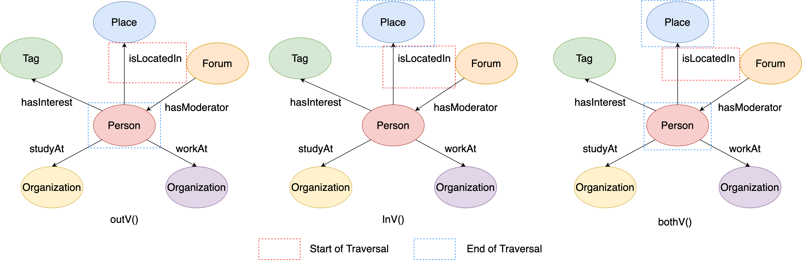
Figure 11. The examples of outV/inV/bothV steps.
Therefore, the output of the above codes should like:
# q1: the edge's outgoing vertex
[v[216172782113784483]]
# q2: the edge's incoming vertex
[v[288230376151712472]]
# q3: both of the edge's outgoing and incoming vertices
[v[216172782113784483], v[288230376151712472]]
For otherV(), it will only traverse to the vertices that haven’t been reached in the traversal history. For example, the ‘isLocatedIn’ edge is reached from the outgoing vertex ‘Person’, then the otherV() of ‘isLocatedIn’ edge is its incoming vertex ‘Place’, because it hasn’t been visited before.
# Traverse from the edge to its incident vertex that hasn't been reached
q1 = g.execute('g.V(216172782113784483).outE("isLocatedIn").otherV()')
print(q1.all().result())
The output should be like:
# q1: 'place' vertex, which has not been reached before
[v[288230376151712472]]
Multiple Expansion Steps
You may have already noticed that graph traversal supports multiple expansion steps. For example, in Gremlin sentenceg.V(216172782113784483).outE('isLocatedIn').inV(), outE('isLocatedIn') is first expansion and inV() is the second expansion.
The figure illustrates the execution process of this Gremlin sentence:
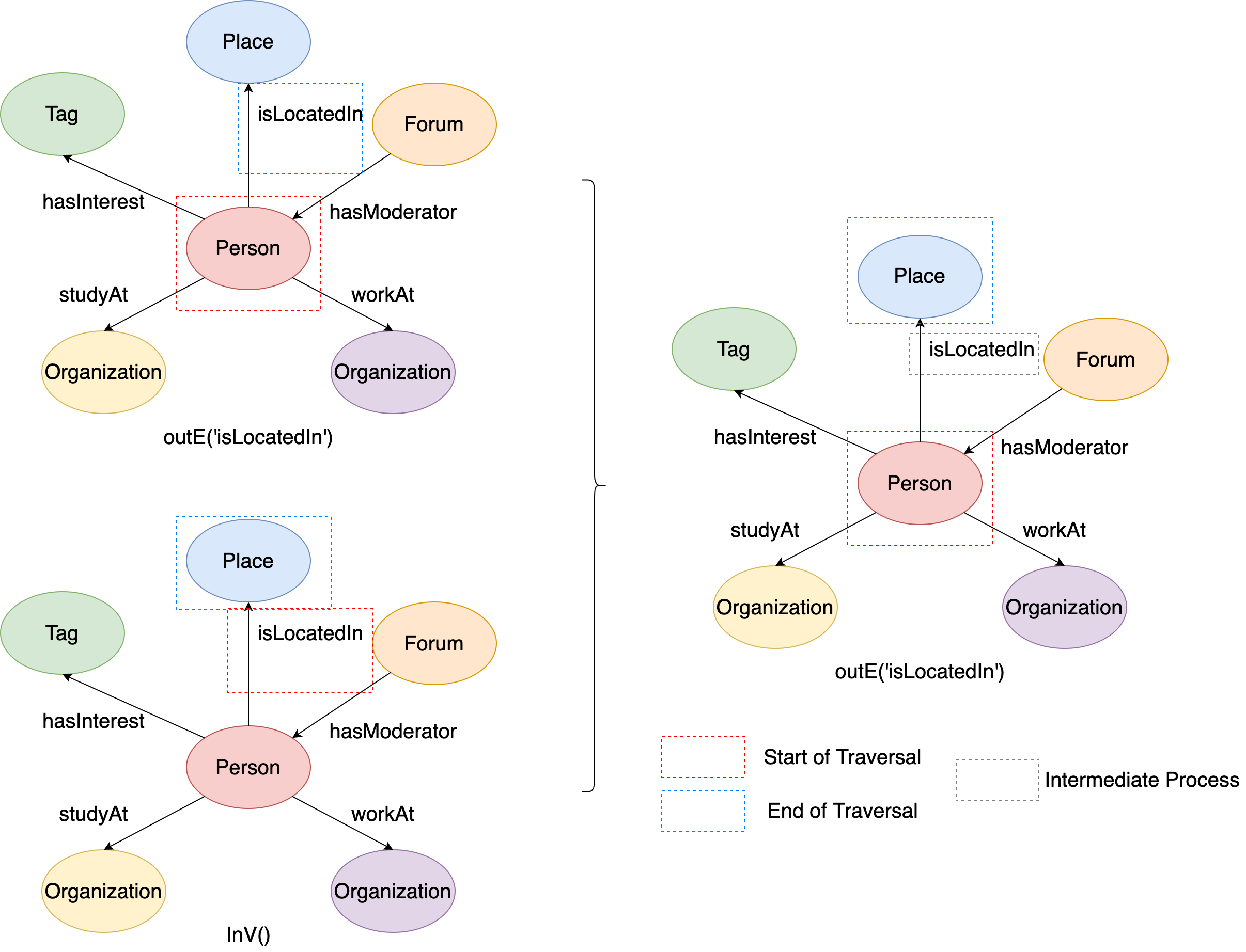
Figure 12. The examples of outE followed by inV.
During the traversal, it firstly start from the source vertex ‘person’, and get to the ‘isLocatedIn’ edge. Then it starts from the ‘isLocatedIn’ edge, and get to the ‘place’ vertex. Thus the traversal ends, the ‘place’ vertex is the end of this traversal, and the ‘isLocatedIn’ edge can be regarded as the intermediate process of the traversal.
When GIE handle continuous multiple expansion steps during the traversal, the next expansion step will use the its previous expansion step’s output as its starting points. According to this property, we can summarize the following equivalent rules:
out() = outE().inV() = outE().otherV()in() = inE().outV() = inE().otherV()both() = bothE().otherV()
It is sure that GIE can support multiple vertex expansion steps. For example, the place (city) the person is located in ‘isPartOf’ a larger place (country). If you want to find the larger place, you can write multiple vertex expansion steps in GIE as:
# Traverse from the vertex to the larger place it is located in by two vertex expansions
q1 = g.execute('g.V(216172782113784483).out("isLocatedIn").out("isPartOf")')
print(q1.all().result())
This figure illustrates the execution process:
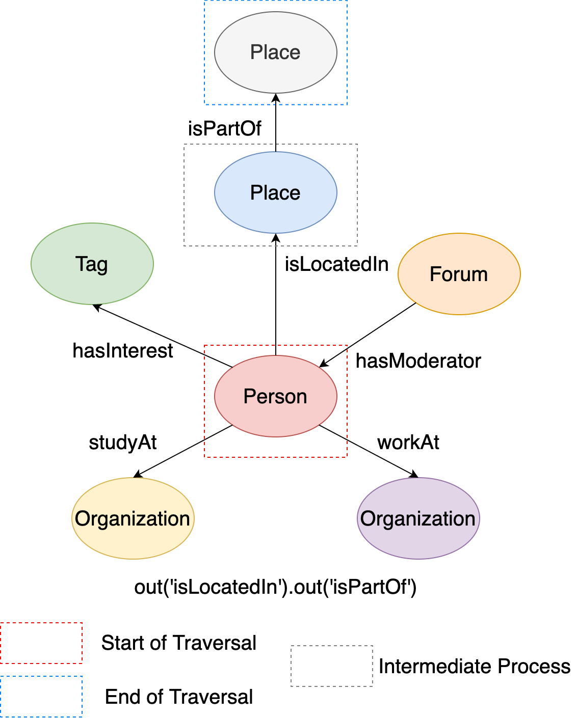
Figure 13. The examples of two-hop outgoing vertices.
Therefore, the output of the Gremlin sentence should be like:
# The larger place(country) that the person is located in
[v[288230376151711797]]
There is one problem of currently introduced Gremlin traversal sentences: only the last step’s results are kept. Sometimes, you may need to record the intermediate results of the traversal for further analysis, but how? Actually, you can use the as(TAG) and select(TAG 1, TAG 2, ..., TAG N) steps to keep the intermediate results:
as(TAG): it gives a tag to the step it follows, and then its previous step’s value can be accessed through the tag.select(TAG 1, TAG 2, ..., TAG N): select all the values of the steps the given tags refer to.
Extend from previous example, if you want to keep person, smaller place(city) and larger place(country) together in the output, you can write Gremlin sentence in GIE like:
# a: person, b: city, c: country
q1 = g.execute('g.V(216172782113784483).as("a")\
                 .out("isLocatedIn").as("b")\
                 .out("isPartOf").as("c")\
                 .select("a", "b", "c")')
print(q1.all().result())
where tag ‘a’ refers to ‘person’ vertex, tag ‘b’ refers to ‘city’ vertex and tag ‘c’ refers to ‘country’ vertex. The output should be like:
[{'a': v[216172782113784483], 'b': v[288230376151712472], 'c': v[288230376151711797]}]
Expansion from many starting points
Currently, we only discuss the expansion from only one vertex/edges. However, it is very common to write Gremlin sentence like g.V().out() in GIE. In previous tutorials we have known that g.V() will get all the vertices in the graph. Then how to understand the meaning of g.V().out()?
The explain it more clear, let’s firstly look at a much simpler situation: starting from only two vertices. This is a subgraph of LDBC Graph formed by two person vertices’ local graphs, where the two person vertices’ ids are 216172782113784483 and 216172782113784555.
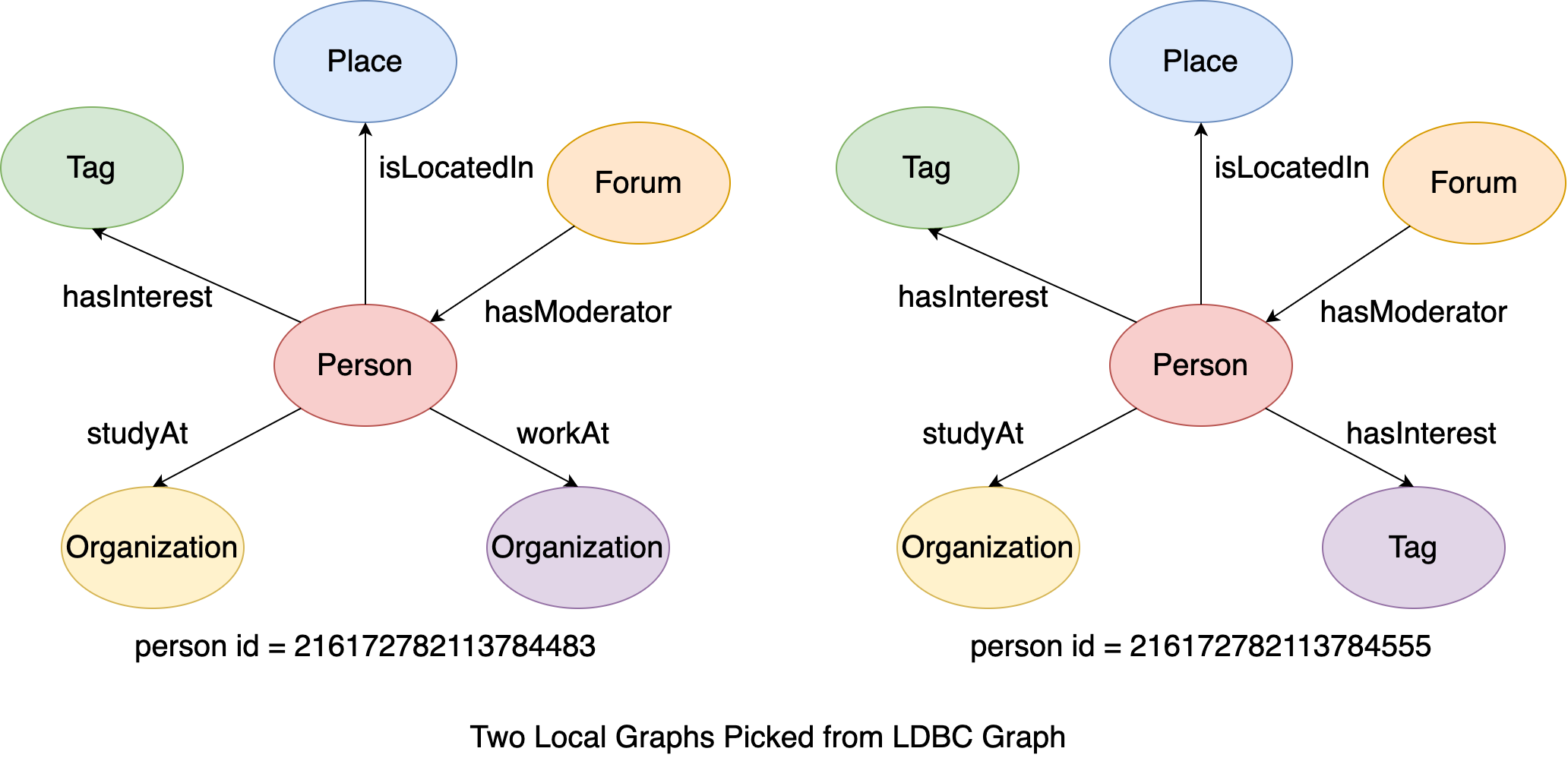
Figure 14. The examples of two local graphs.
In addition, we further limit the starting points of the traversal to be exactly the two person vertices. Therefore, we can write the following Gremlin sentence in GIE:
# Traverse from the two source vertices to their adjacent vertices through their incident outgoing edges
q1 = g.execute('g.V(216172782113784483, 216172782113784555).out()')
print(q1.all().result())
The figure illustrates the execution process of q1:
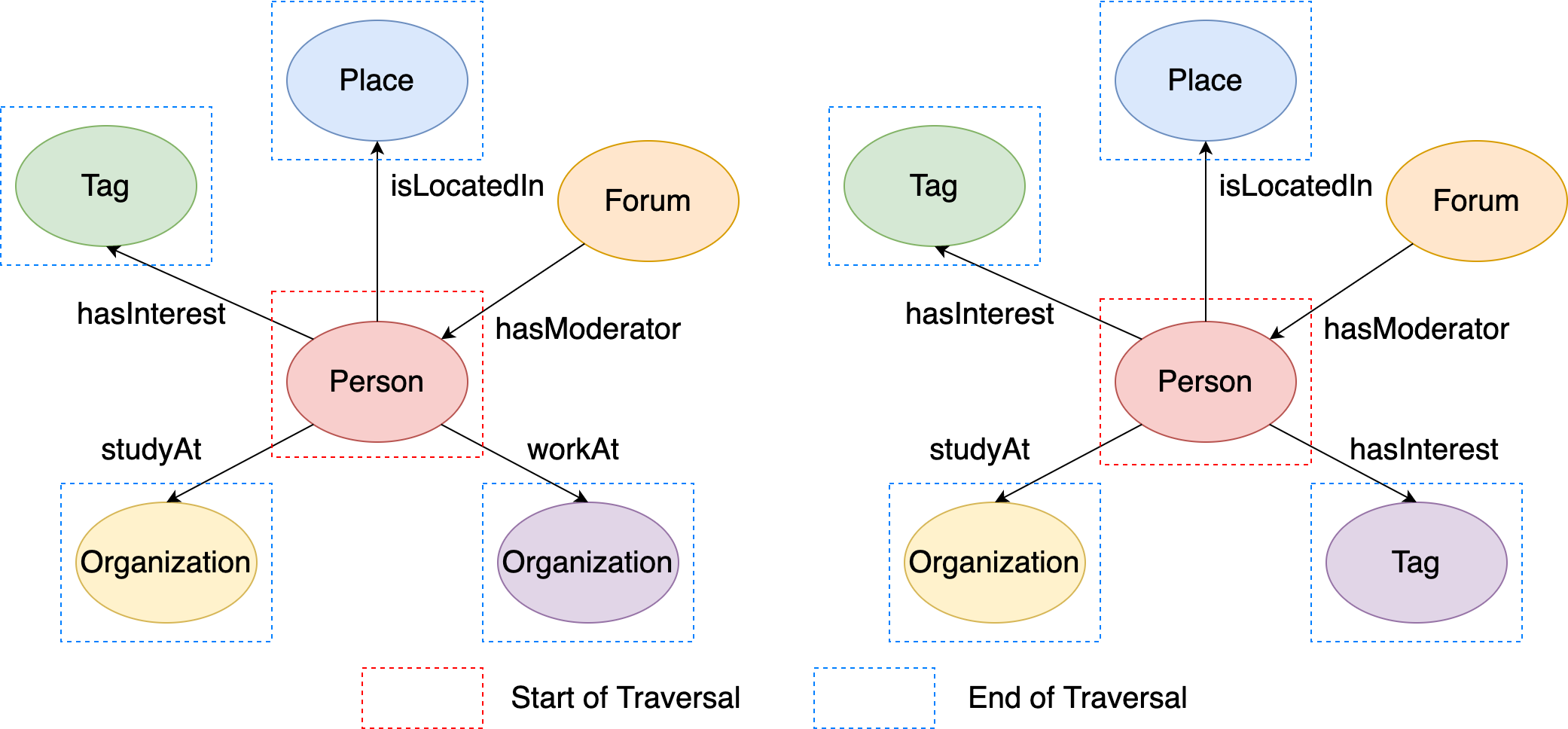
Figure 15. The results of outgoing neighbors from two given vertices.
The traversal starts from the two person vertices, and then the out() step map the two source vertices both to their outgoing adjacent vertices. Therefore, the output should be like:
[v[432345564227569033], v[288230376151712472], v[144115188075856168], v[144115188075860911], v[432345564227569357], v[432345564227570524], v[288230376151712984], v[144115188075861043]]
which are the outgoing adjacent vertices of the two ‘person’ vertices.
It is more clear to understand if you keep person vertex’s info in the final output:
q1 = g.execute('g.V(216172782113784483, 216172782113784555).as("a")\
                 .out().as("b")\
                 .select("a", "b")')
print(q1.all().result())
# the first 4 elements are tuple of vertex(id=216172782113784483) and its outgoing adjacent vertex
# the last 4 elements are tuple of vertex(id=216172782113784555) and its outgoing adjacent vertex
[{'a': v[216172782113784483], 'b': v[432345564227569033]},
 {'a': v[216172782113784483], 'b': v[288230376151712472]},
 {'a': v[216172782113784483], 'b': v[144115188075856168]},
 {'a': v[216172782113784483], 'b': v[144115188075860911]},
 {'a': v[216172782113784555], 'b': v[432345564227569357]},
 {'a': v[216172782113784555], 'b': v[432345564227570524]},
 {'a': v[216172782113784555], 'b': v[288230376151712984]},
 {'a': v[216172782113784555], 'b': v[144115188075861043]}]
Generally, it is better to understand the expansion and traversal step from traverser’s aspect. Every expansion step actually map current traversers to another series traversers, and the complete traversal can be regarded as the transformations of traversers. Let’s take g.V().out().in() as an example to explain it.
At the very beginning,
g.V()extracts all the vertices from the graph, and these vertices form the initial traversers: each traverser contains the corresponding vertex.Then
out()maps every traverser (vertex) to its outgoing adjacent vertices, and these outgoing adjacent vertices form the next series of traversers.Finally,
in()maps every traverser (vertex) to its incoming adjacent vertices, and these incoming adjacent vertices form the next series of traversers, and it is the final output of the Gremlin sentence.
This figure illustrates the overview of the traverser transformation during the traversal of g.V().out().in().
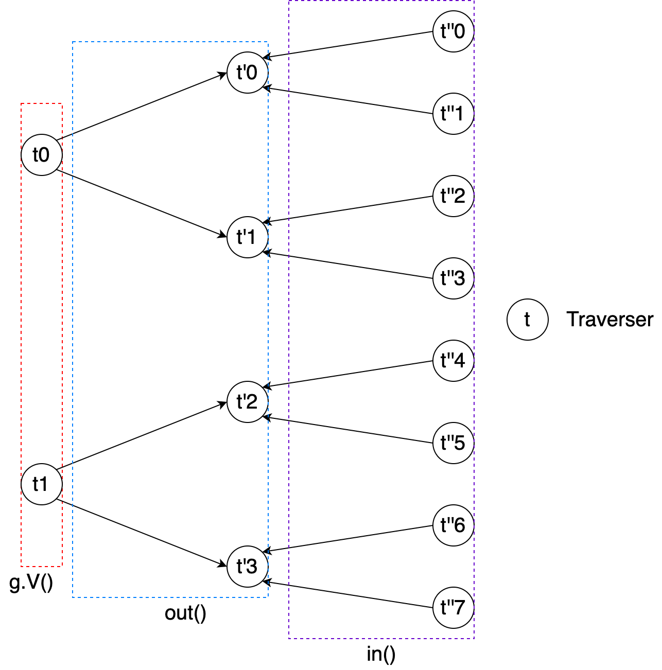
Figure 16. The overview of traversers’ transformation.
In addition, this figure shows the details of the traverser’s change after every expansion step and as(TAG) step during the execution of Gremlin sentence g.V().as('a').out().as('b').in().as('c').
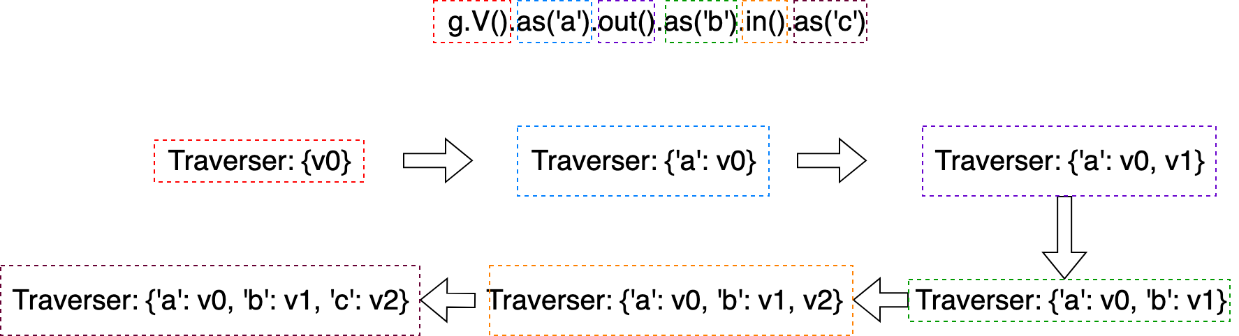
Figure 17. The mapping details of the above traversers’ transformation.
Filter & Expansion
Apply filters after expansion
In last tutorial, we have discussed that we can use has(...) series of steps to apply filters to the extracted vertices and edges. Actually, these steps can be applied after expansion steps either that filter on the current traversers.
Still using g.V().out().in() as the example, if we hope that:
The traversers(vertices) after
g.V()has label ‘person’The traversers(vertices) after the first expansion
out()have property ‘browserUsed’ and the value is ‘Chrome’The traversers(vertices) after the second expansion
in()have property ‘length’ and the length is < 5, and the label of the expansion edge is ‘replyOf’
# Traversers(vertices) after g.V() has label 'person'
# Traversers(vertices) after out() has property 'browserUsed' and the value is 'Chrome'
# Traversers(vertices) after in('replyOf') has property 'length' and the length is < 5
q1 = g.execute('g.V().hasLabel("person")\
                     .out().has("browserUsed", "Chrome")\
                     .in("replyOf").has("length", lt(5))')
print(q1.all().result())
The output should be like:
[v[54336], ..., v[33411]]
Furthermore, for Gremlin sentences contain as(TAG) steps, we can introduce where() step to apply filters on traversers based on the tagged values.
Extend from previous example that we add tag ‘a’ and ‘b’ after the two has(...) step:
q1 = g.execute('g.V().hasLabel("person")\
                     .out().has("browserUsed", "Chrome").as("a")\
                     .in("replyOf").has("length", lt(5)).as("b")')
If we hope that the vertices of the tag ‘a’ and ‘b’ have the same property value on property ‘browserUsed’, we can add a where step and write the following Gremlin sentence in GIE:
# Traversers(vertices) after g.V() has label 'person'
# Traversers(vertices) after out() has property 'browserUsed' and the value is 'Chrome'
# Traversers(vertices) after in('replyOf') has property 'length' and the length is < 5
# vertex a and b have the same value of 'browserUsed' property
q1 = g.execute('g.V().hasLabel("person")\
                     .out().has("browserUsed", "Chrome").as("a")\
                     .in("replyOf").has("length", lt(5)).as("b")\
                     .where("b", eq("a")).by("browserUsed")\
                     .select("a", "b")')
print(q1.all().result())
print(q1.all().result())
The output should be like:
[{'a': v[360287970189700805], 'b': v[59465]}, ..., {'a': v[33403], 'b': v[33411]}]
Expansion as filters
In addition, not only can we add filters after expansion steps, but also we can use expansion step as the filtering predicate with where(...) step. For example, if we want to extract all the vertices having at least 5 outgoing incident edges, we can write a Gremlin sentence with where(...) step as following:
# Retrieve vertices having at least 5 outgoing incident edges
q1 = g.execute('g.V().where(outE().count().is(gte(5)))')
print(q1.all().result())
Path Expansion (Syntactic Sugar)
Until now, we can use expansion steps, filter steps and auxiliary steps like as(TAG) to write complicated Gremlin sentences to traverse the graph. However, there are still two shortcomings:
If we want to find a vertex which is 10-hop(edges) away from the current vertex, we need to write expansion step 10 times, which is very cost-ineffective.
The number of hops from the source to the destination is arbitrary. For example, if we want to find all vertices which can be reached from a source vertex within 3-hops, it cannot be solved by already introduced steps.
Therefore, we would like to introduce path expansion to solve the two problems, which extends the expansion steps out(), in() and both() as the syntactic sugar.
In the three expansion steps, you can now write as out/in/both(lower..upper, label1, label2...), where lower is the minimum number of hops in the path, and upper-1 is the maximum number of hops in the path. For example, out(3..5) means expansion through the outgoing edges 3 or 4 times. Therefore, lower <= upper - 1, otherwise the sentence is illegal.
Path expansion is very flexible. Therefore, we design the with() step followed by path expansion step to provide two options for user to configure the corresponding behaviors of the path expansion step:
PATH_OPT: Since path expansion allows expand the same step multiple times, it is likely to have duplicate vertices in the path. If thePATH_OPTis set toARBITRARY, paths having duplicate vertices will be kept in the traversers; otherwise, if thePATH_OPTis set toSIMPLE_PATH, paths having duplicate vertices will be filtered.RESULT_OPT: Sometimes, you may be interested in all the vertices in the path, but sometimes you may be only interested in the last vertex of the path. Therefore, when theRESULT_OPTis set toALL_V, all the vertices in the path will be kept to the output. Instead, when theRESULT_OPTis set toEND_V, only the last vertex of the path will be kept.
At last, we would like to introduce endV() step in path expansion. Since a path may contain many vertices, all kept vertices are stored in a path collection by default. Therefore, endV() is used to unfold the path collection. For example, if the traversers after path expansion is [[v[1], v[2], v[3]], where the inner [v[1], v[2], v[3]] is the path collection. With the endV(), v[1], v[2] and v[3] are picked out from the path collection, and the traversers becomes [v[1], v[2], v[3]]
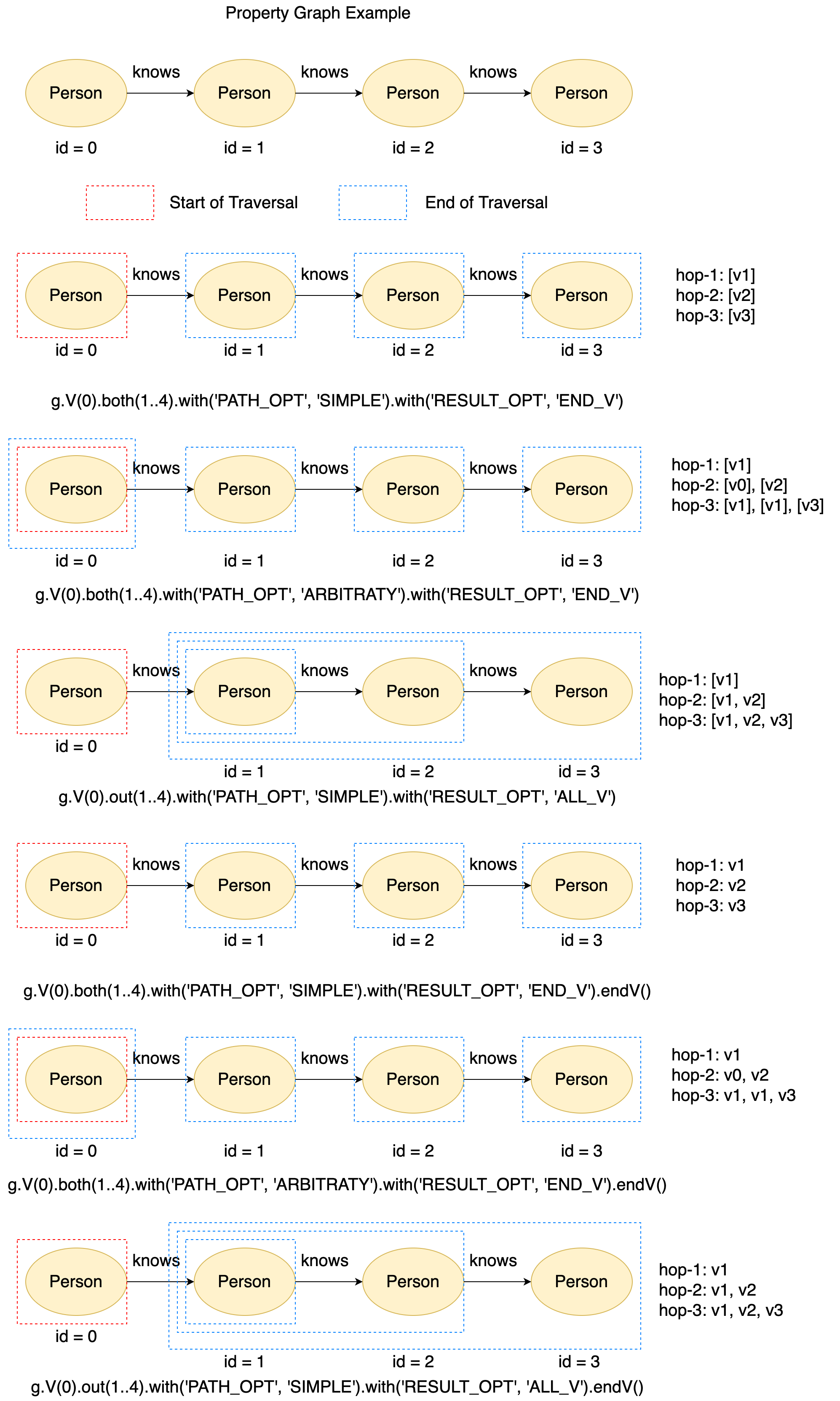
Figure 18. The examples of path expansion.
Real Applications
Graph traversal enables us to conduct more complicated data analytics on the graph.
For example, the path comment-hasCreator->person->isLocatedIn->city-isPartOf->country can help to determine the nationality of comments. Therefore, we can calculate the histogram of comment length for comments from China easily with GIE:
import matplotlib.pyplot as plt
import numpy as np
import graphscope as gs
from graphscope.dataset.ldbc import load_ldbc

# load the modern graph as example.
graph = load_ldbc()

# Hereafter, you can use the `graph` object to create an `gremlin` query session
g = gs.gremlin(graph)
# Extract all comments' contents in China
q1 = g.execute('g.V().hasLabel("person").where(out("isLocatedIn").out("isPartOf").values("name").is(eq("China"))).in("hasCreator").values("content")')
comment_contents = q1.all()
comment_length = [len(comment_content.split()) for comment_content in comment_contents];

plt.hist(x=list(filter(lambda x:(x< 50), comment_length)), bins='auto', color='#607c8e',alpha=0.75)
plt.grid(axis='y', alpha=0.75)
plt.xlabel('Comments Length')
plt.ylabel('Comments Count')
plt.title('Comment Length Histogram for comments from China')
plt.show()
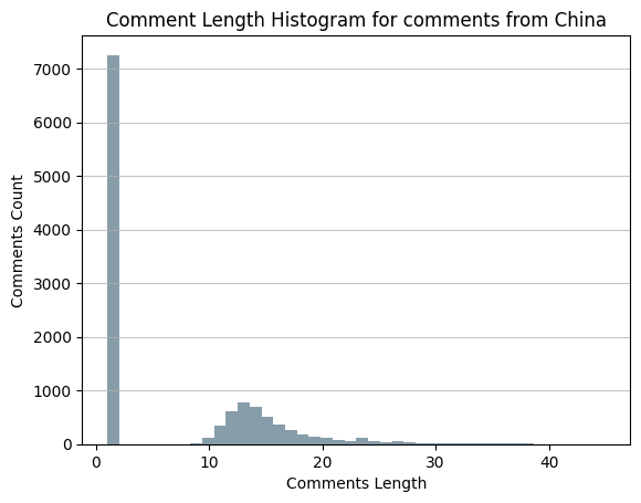
Figure 19. Comments length histogram in China.
Or we can estimate the browser market share in Japan:
import matplotlib.pyplot as plt
import graphscope as gs
from graphscope.dataset.ldbc import load_ldbc
from collections import Counter


# load the modern graph as example.
graph = load_ldbc()

# Hereafter, you can use the `graph` object to create an `gremlin` query session
g = gs.gremlin(graph)

# Extract all person' gender property value
q1 = g.execute('g.V().hasLabel("person").where(out("isLocatedIn").out("isPartOf").values("name").is(eq("Japan"))).in("hasCreator").values("browserUsed")')
browsers_used = q1.all()
browser_list = ['Firefox', 'Chrome', 'Internet Explorer', 'Safari']
# Count Firefox, Chrome, Internet Explorer and Safari
browser_counts = Counter(browsers_used)

# Draw pie chart
plt.pie(x=[browser_counts[browser] for browser in browser_list], labels=browser_list, autopct='%1.1f%%')
plt.show()
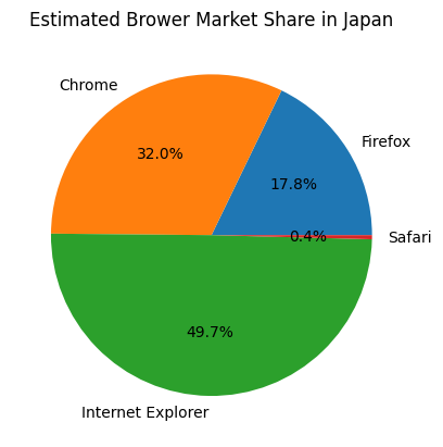
Figure 20. Estimated Japan Browser Market Share
Pattern Match
Suppose you want to find two persons and the universities they studyAt in the graph that:
The two
personknoweach otherThe two
personstudyAtthe sameuniversity
With the method taught previously , you can write the following code in GIE to achieve this purpose:
q1 = g.execute('g.V().hasLabel("person").as("person1").both("knows").as("person2")\
                     .select("person1").out("studyAt").as("university1")\
                     .select("person2").out("studyAt").as("university2")\
                     .where("university1", eq("university2"))\
                     .select("person1", "person2", "university1")')
print(q1.all().result())
First, you find all pairs of
person1andperson2who know each other.Then, you find
person1’s university asuniversity1andperson2’s university asuniversity2.Next, you use the
where(...)step to check whetheruniversity1is equal touniversity2and filter out those that are not equal.Finally, you use the
select(...)step to projectperson1,person2, anduniversity1(nowuniversity1is the same asuniversity2).
The output of should be like:
# Person1 and 2 know each other and study at the same university
[{'person2': v[216172782113784481],
  'person1': v[216172782113784279],
  'university1': v[144115188075858884]},
 {'person2': v[216172782113784361],
  'person1': v[216172782113784291],
  'university1': v[144115188075858879]},
 {'person2': v[216172782113784642],
  'person1': v[216172782113784291],
  'university1': v[144115188075858879]},
 {'person2': v[216172782113784473],
  'person1': v[216172782113784328],
  'university1': v[144115188075858700]},
 {'person2': v[216172782113784700],
  'person1': v[216172782113784331],
  'university1': v[144115188075860619]},
 {'person2': v[216172782113784375],
  'person1': v[216172782113784333],
  'university1': v[144115188075858813]},
 {'person2': v[216172782113784593],
  'person1': v[216172782113784361],
  'university1': v[144115188075858879]},
 {'person2': v[216172782113784642],
  'person1': v[216172782113784361],
  'university1': v[144115188075858879]},
 {'person2': v[216172782113784291],
...
  'person1': v[216172782113784688],
  'university1': v[144115188075860870]},
 {'person2': v[216172782113784047],
  'person1': v[216172782113784692],
  'university1': v[144115188075862429]}]
Actually, such kind of problem is called graph pattern matching. It means, you define a pattern at first. The pattern can be either described by the natural language:
“Find two
personsand theuniversitiestheystudyAtin the graph that the twopersonknoweach other and the twopersonstudyAtthe sameuniversity”
or can be illustrated as a graph pattern as shown in the following.
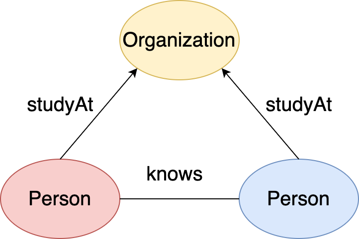
Figure 21. Pattern: two person know each other and study at the same university.
Then you aim to find all the matched subgraphs that are isomorphic to the pattern. Under graph isomorphism, a subgraph and the pattern are matched if, when there is an edge between vertices in the pattern, there is an equivalent edge between two matched vertices in the subgraph. In addition, a vertex in the subgraph cannot match multiple pattern vertices.
For example, this is a local graph of university vertex(id = 144115188075858884) in the LDBC Graph:
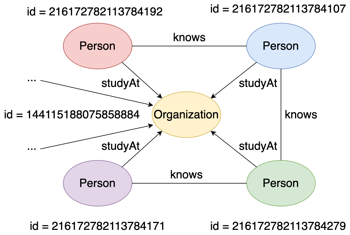
Figure 22. Local graph of a university vertex.
and here are the matched subgraphs in this local graph:
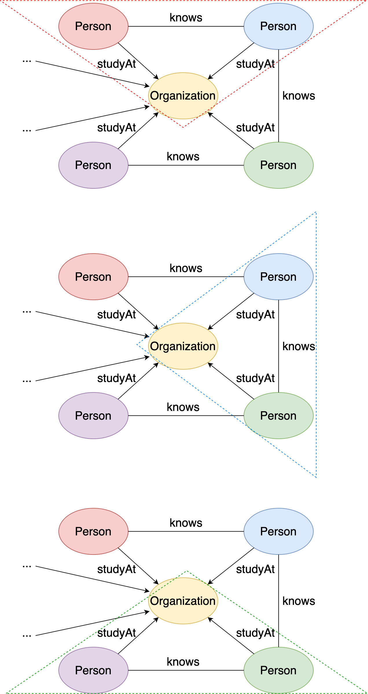
Figure 23. Three matched subgraphs in the local graph.
The matched instances in the local graph are:
{person1: v[216172782113784192], person2: v[216172782113784107], university: v[144115188075858884]}{person1: v[216172782113784107], person2: v[216172782113784192], university: v[144115188075858884]}{person1: v[216172782113784107], person2: v[216172782113784279], university: v[144115188075858884]}{person1: v[216172782113784279], person2: v[216172782113784107], university: v[144115188075858884]}{person1: v[216172782113784279], person2: v[216172782113784171], university: v[144115188075858884]}{person1: v[216172782113784171], person2: v[216172782113784279], university: v[144115188075858884]}
There are a total of 6 matched instances (compared to 3 subgraphs) because changing the position of person1 and person2 leads to a new matched instance.
As shown at the beginning of this section, you can write a regular Gremlin query to conduct pattern matching. However, it has two shortcomings:
The query sentence is complex. If you write such a long query sentence for this simple triangle pattern, what about more complicated patterns like squares, butterflies, or cliques?
There’s almost no optimization. The speed of pattern matching largely depends on how you write the query sentence.
To solve these two problems, GIE supports the match(...) step in Gremlin, which is specifically designed for pattern matching.
The match() step provides a more declarative form of graph querying based on the notion of pattern matching:
Every
match()step is a collection ofsentences, and everysentenceis a regular Gremlin traverser sentence but starts and ends with given tags.Then, GIE uses the underlying MatchAnalyticsAlgorithm to connect all the
sentencestogether to form a pattern structure based on those start and end tags.Finally, GIE applies its MatchOptimizationAlgorithm to generate an optimized matching strategy for the formed pattern and conduct the pattern matching.
Therefore, it is much more efficient to solve pattern matching problems using Gremlin’s built-in match() step.
As for the pattern shown at the beginning of this section (two persons who know each other and study at the same university), you can write the following code in GIE using the match() step:
# Person1 and 2 know each other and study at the same university
q1 = g.execute('g.V().match(__.as("person1").both("knows").as("person2"),\
                       __.as("person1").out("studyAt").as("university"),\
                       __.as("person2").out("studyAt").as("university"))')
print(q1.all().result())
The output should be the same as the previous self-written pattern matching sentences:
[{'person2': v[216172782113784361],
  'person1': v[216172782113784291],
  'university': v[144115188075858879]},
 {'person2': v[216172782113784642],
  'person1': v[216172782113784291],
  'university': v[144115188075858879]},
 {'person2': v[216172782113784375],
  'person1': v[216172782113784333],
  'university': v[144115188075858813]},
 {'person2': v[216172782113784593],
  'person1': v[216172782113784361],
  'university': v[144115188075858879]},
 {'person2': v[216172782113784642],
  'person1': v[216172782113784361],
  'university': v[144115188075858879]},
 {'person2': v[216172782113784587],
  'person1': v[216172782113784363],
  'university': v[144115188075860919]},
 {'person2': v[216172782113784532],
  'person1': v[216172782113784400],
  'university': v[144115188075861858]},
 {'person2': v[216172782113784491],
  'person1': v[216172782113784401],
  'university': v[144115188075858086]},
 {'person2': v[216172782113784598],
...
  'person1': v[216172782113784629],
  'university': v[144115188075858881]},
 {'person2': v[216172782113783931],
  'person1': v[216172782113784657],
  'university': v[144115188075858708]}]
Let’s present a more complex pattern matching example: we want to find two persons A and B such that:
they know each other
personA creates amessage, which is replied to by acommentcreated bypersonB
This figure illustrates the pattern:
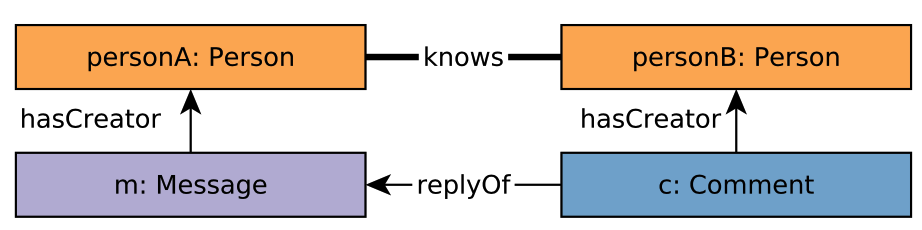
Figure 24. Pattern: two person know each other, and one person creates a comment replying a message created by the other.
We can easily match this pattern with Gremlin match(...) step:
# pA and pB know each other
# pB create a comment that reply a message created by pA
q1 = g.execute('g.V().match(__.as("pA").both("knows").as("pB"),\
                       __.as("pA").in("hasCreator").as("m"),\
                       __.as("pB").in("hasCreator").as("c"),\
                       __.as("c").out("replyOf").as("m"))')
print(q1.all().result())
The output should be like:
[{'pA': v[216172782113783809], 'pB': v[216172782113784011], 'c': v[3], 'm': v[360287970189640007]}, {'pA': v[216172782113783809], 'pB': v[216172782113784011], 'c': v[4], 'm': v[360287970189640007]}, {'pA': v[216172782113783809], 'pB': v[216172782113784011], 'c': v[5], 'm': v[360287970189640007]}, {'pA': v[216172782113783809], 'pB': v[216172782113784011], 'c': v[13], 'm': v[360287970189640007]}, {'pA': v[216172782113783809], 'pB': v[216172782113784011], 'c': v[18], 'm': v[360287970189640007]}, {'pA': v[216172782113783809], 'pB': v[216172782113784011], 'c': v[19], 'm': v[360287970189640007]}, {'pA': v[216172782113783809], 'pB': v[216172782113784011], 'c': v[22], 'm': v[360287970189640008]}, {'pA': v[216172782113783809], 'pB': v[216172782113784011], 'c': v[27], 'm': v[360287970189640008]}, {'pA': v[216172782113783809], 'pB': v[216172782113784011], 'c': v[29], 'm': v[360287970189640009]}, {'pA': v[216172782113783809], 'pB': v[216172782113784011], 'c': v[34], 'm': v[360287970189640009], ......, }]
Note that every match sentence inside the match(...) step supports filter steps and path expands. For example, if you hope that the knows edge is a 1..3 multi-hop, and the message and comment are created after 2012-01-01, you can write:
# pA and pB know each other
# pB create a comment that reply a message created by pA
q1 = g.execute('g.V().match(__.as("pA").both("1..3", "knows").as("pB"),\
                       __.as("pA").in("hasCreator").has("creationDate", gt("2012-01-01")).as("m"),\
                       __.as("pB").in("hasCreator").has("creationDate", gt("2012-01-01")).as("c"),\
                       __.as("c").out("replyOf").as("m"))')
print(q1.all().result())
The output should be like:
[{'pA': v[216172782113783812], 'pB': v[216172782113783882], 'c': v[36], 'm': v[360287970189640010]}, {'pA': v[216172782113783812], 'pB': v[216172782113783882], 'c': v[37], 'm': v[360287970189640010]}, {'pA': v[216172782113783812], 'pB': v[216172782113784105], 'c': v[38], 'm': v[360287970189640010]}, {'pA': v[216172782113783812], 'pB': v[216172782113783882], 'c': v[41], 'm': v[360287970189640010]}, {'pA': v[216172782113784105], 'pB': v[216172782113783882], 'c': v[43], 'm': v[42]}, {'pA': v[216172782113783814], 'pB': v[216172782113783962], 'c': v[50], 'm': v[360287970189640135]}, {'pA': v[216172782113783814], 'pB': v[216172782113784171], 'c': v[52], 'm': v[360287970189640135]}, {'pA': v[216172782113784481], 'pB': v[216172782113784199], 'c': v[54], 'm': v[49]}, {'pA': v[216172782113783814], 'pB': v[216172782113784038], 'c': v[56], 'm': v[360287970189640135]}, {'pA': v[216172782113783816], 'pB': v[216172782113784144], 'c': v[175], 'm': v[360287970189640462], ......, }]
Relational Operations
Then we would like to introduce more relational operations of Gremlin steps that GIE supports.
Filter Steps
hasId()
In previous tutorial, we have introduced that you can use g.V(id) to pick out the vertex having specific required global id from the graph. But, what if we want to apply filters based on global id during the traversal?
You can use the hasId(id) step to achieve the purpose. For example, if you want the expanded vertex exactly having global id 144115188075861858, you can write the following codes in GIE:
q1 = g.execute('g.V().out().hasId(144115188075861858)')
print(q1)
The output should be like:
[v[144115188075861858], v[144115188075861858], v[144115188075861858]]
Note that hasId(id) is different from has('id', id)! As mentioned before, hasId(id) apply filter based on the global id, while has('id', id) apply filter based on the local id. For example, if you write:
q1 = g.execute('g.V().has("id", 0)')
print(q1.all().result())
The output would be:
[v[72057594037927936],
 v[144115188075855872],
 v[288230376151711744],
 v[432345564227567616],
 v[504403158265495555]]
which are all the vertices whose local id is 0.
where()
In previous tutorial, we have introduced that where() step in Gremlin sentences having as() steps can be used to filter traversers based on the tagged values:
# vertex tagged as 'a' should be the same as vertex 'tagged' as b
q1 = g.execute('g.V(216172782113783808).as("a")\
                 .out("knows").in("knows").as("b").where("b", P.eq("a"))')
print(q1.all().result())
The output should be like:
[v[216172782113783808], v[216172782113783808], v[216172782113783808]]
In addition, where() step can be followed by a by(...) step to provide much more powerful functionalities: the selected entities may not need to compare themselves, but compare their properties.
For example, the following Gremlin sentence require vertex ‘a’ and ‘b’ having the value on same ‘firstName’ :
# vertex tagged as 'a' and 'b' should have the same property 'name'
q1 = g.execute('g.V(216172782113783808).as("a").out("knows").in("knows").as("b")\
                 .where("b", P.eq("a")).by("firstName")')
print(q1.all().result())
The output should also be like:
[v[216172782113783808], v[216172782113783808], v[216172782113783808]]
In addition, if you hope that vertex ‘a’ and ‘b’ having the same output degree, you can write:
# vertex tagged as 'a' and 'b' should have the output degree
q1 = g.execute('g.V(216172782113783808).as("a").out("knows").in("knows").as("b")\
                 .where("b", P.eq("a")).by(out().count())')
print(q1.all().result())
The output should be like:
# v[216172782113784171] is not v[216172782113783808](the source vertex),
# but have the same output degree
[v[216172782113783808], v[216172782113783808], v[216172782113783808], v[216172782113784171]]
dedup()
Suppose that you are interested in how many forums having members from India, and you may write the following Gremlin sentence in GIE:
# Aim to count how may forums have members from India
q1 = g.execute('g.V().hasLabel("place").has("name", "India")\
                 .in("isPartOf").in("isLocatedIn").in("hasMember").count()')
print(q1.all().result())
The output is [8248]. It seems to have no problem. However, how many forums are there in the graph?
# Count how many forums are there in the graph
q1 = g.execute('g.V().hasLabel("forum").count()')
print(q1.all().result())
The output is [8101]. Here comes the problem: the number of forums having members from India is even larger than the total number of forums. It is impossible! Actually, when we count how many forums having members from India with previous graph traversal, the last step .in(\'hasMember\') will lead to many duplicates, because it is very common for different people to join the same forum.
Therefore, dedup() step is designed to remove the duplicates among traversers. After we add the dedup() step before the count(), the statistics result is back to normal:
# Count how may forums have members from India
q1 = g.execute('g.V().hasLabel("place").has("name", "India")\
                 .in("isPartOf").in("isLocatedIn").in("hasMember").dedup().count()')
print(q1.all().result())
The output is [2822].
For Gremlin sentence containing as() step, we can also dedup(TAG) remove duplicates according to specific tagged entities. For example, the following Gremlin sentence also counts how may forums have members from India, but the traverser starts from forum. To remove the duplicates, we dedup('a'), where ‘a’ is the taggedforum vertices.
# Count how may forums have members from India
q1 = g.execute('g.V().hasLabel("forum").as("a").out("hasMember")\
                     .out("isLocatedIn").out("isPartOf").has("name", "India")\
                     .dedup("a").count()')
print(q1)
The output is also [2822].
In addition, we can dedup(TAG1, TAG2, ...) to remove duplicates by the composition of several tagged entires. For example, the following Gremlin sentence counts there are how many different related (country, forum) pairs in the graph.
# Count how many different related (country, forum) pairs in the graph
q1 = g.execute('g.V().hasLabel("place").as("a")\
                 .in("isPartOf").in("isLocatedIn")\
                 .in("hasMember").as("b").dedup("a", "b").count()')
print(q1.all().result())
The output is [37164]
Furthermore, just like previously introduced where() step, we can add by(...) after dedup(...) step to remove duplicates based on the property values. For example, if you want to count there are how many different firstNames of persons in the graph, you can write in GIE as:
# Count how many different firstName are there in the graph
q1 = g.execute('g.V().hasLabel("person").dedup().by("firstName").count()')
print(q1)
The output should be [432].
Project Steps
id() and label()
In previous tutorial, we have taught to use values(PROPERTY) to project an entity (vertex or edge) to its property’s value. However, to extract the global id and label, we may need to separate steps: id() and label():
# Get vertex(id=72057594037927936) ’s id
q1 = g.execute('g.V(72057594037927936).id()')
# Get vertices(label='person')'s label
q2 = g.execute('g.V().hasLabel("person").label()')

print(q1.all().result())
print(q2.all().result())
The output should be like:
# ID
[72057594037927936]
# Labels
[3, ..., 3]
Note that id() step is not equivalent to values("id"), where the latter one project an entity (vertex or edge) to its local id! For example:
# Get vertex(id=72057594037927936) ’s local id
q1 = g.execute('g.V(72057594037927936).values("id")')
print(q1.all().result())
The output is [0]
constant()
The constant() step is meant to map any object to a fixed object value. For example:
# Map all the vertices to 1
q1 = g.execute('g.V().constant(1)')
# Map all the vertices to "marko"
q2 = g.execute('g.V().constant("marko")')
# Map all the vertices to 1.0
q3 = g.execute('g.V().constant(1.0)')
print(q1.all().result())
print(q2.all().result())
print(q3.all().result())
The output should be like:
# 1s
[1, ..., 1]
# "markos"
["marko", ..., "marko"]
# 1.0s
[1.0, ..., 1.0]
valueMap()
value(PROPERTY) step can only map an entity(vertex or edge) to one of its property’s value. What if we want to extract many properties’s value at the same time?
valueMap(PROPERTY1, PROPERTY2, ...) step provides such ability. For example, the following code extracts person vertices’ firstName and lastName together by valueMap(...) step.
# Extract person vertices' firstName and lastName
q1 = g.execute('g.V().hasLabel("person").valueMap("firstName", "lastName")')
print(q1.all().result())
The output should be like:
[{'lastName': ['Donati'], 'firstName': ['Luigi']}, {'lastName': ['Hall'], 'firstName': ['S. N.']},
......
, {'lastName': ['Costa'], 'firstName': ['Carlos']}, {'lastName': ['Khan'], 'firstName': ['Meera']}]
select()
As introduced previously, for a Gremlin sentence containing as() step, we can use select(TAG1, TAG2, ...) step to extract the tagged entities we want. Just as where() and dedup() step, we can add a by(...) step after it to further extract the property’s value of the tagged entities.
For example, the following Gremlin sentence picked the tagged ‘a’ vertex’s firstName.
# Extract tagged 'a' vertex's firstName
q1 = g.execute('g.V().hasLabel("person").as("a").select("a").by("firstName")')
print(q1.all().result())
The output should be like:
['Mahinda', 'Eli', 'Joseph',... ]
Actually, contents inside the by(...) step can be a sub-traversal. For example, the following Gremlin sentence extract tagged ‘a’ vertex’s out degree.
# Extract tagged 'a' vertex's out degree
q1 = g.execute('g.V().hasLabel("person").as("a").select("a").by(out().count())')
print(q1.all().result())
The output should be like:
[36, 12, 94, 228, ...]
In addition, if you want to extract multiple properties’ values of the tagged vertices, you can embed valueMap(TAG1, TAG2, ...) step inside the by(...) step. For example:
# Extract tagged 'a' vertex's firstName and lastName
q1 = g.execute('g.V().hasLabel("person").as("a").select("a").by(valueMap("firstName", "lastName"))')
print(q1.all().result())
The output should be like:
[{'lastName': ['Donati'], 'firstName': ['Luigi']}, {'lastName': ['Hall'], 'firstName': ['S. N.']}, ..., ]
Furthermore, if you want to add by() step after select(TAG1, TAG2, ...) which contains multiple tags, assume the tags number is \(n\), you should add \(n\) by() steps after the select(...) step, and the \(i^{th}\) by() step corresponds to the \(i^{th}\) tag. For example, if you want to extract vertex ‘a’s firstName and vertex ‘b’s lastName, you can write:
# extract vertex 'a's firstName and vertex 'b's lastName
q1 = g.execute('g.V().hasLabel("person").as("a").out("knows").as("b")\
                 .select("a", "b").by("firstName").by("lastName")')
print(q1.all().result())
The output should be like:
[{'a': 'Luigi', 'b': 'Dom Pedro II'}, {'a': 'Luigi', 'b': 'Condariuc'}, {'a': 'Luigi', 'b': 'Bonomi'}, ..., ]
Note that, if select(TAG1, TAG2...) step containing \(n\) tags has by() step followed, then it must be \(n\) by() steps. For some tagged entities, even if we don’t want to project them to anything, we have to give them a corresponding empty by() step. For example, the following code only project vertex ‘b’ to its lastName but leave vertex ‘a’ as it is.
# extract vertex 'a' and vertex 'b's lastName
q1 = g.execute('g.V().hasLabel("person").as("a").out("knows").as("b")\
                 .select("a", "b").by().by("lastName")')
print(q1.all().result())
The output should be like:
[{'a': v[216172782113783808], 'b': 'David'}, {'a': v[216172782113783809], 'b': 'Silva'}, {'a': v[216172782113783809], 'b': 'Guliyev'},..., ]
Aggregate Steps
fold()
Gremlin sentences always generate output containing many traversers. fold() step can roll up these traversers into an aggregate list. For example:
# Roll up the TagClass vertices into an aggregate list
q1 = g.execute('g.V().hasLabel("tagClass").fold()')
print(q1.all().result())
The output should be like:
[[v[504403158265495552], v[504403158265495553], v[504403158265495554], v[504403158265495555], v[504403158265495556], v[504403158265495557], v[504403158265495558], v[504403158265495559], v[504403158265495560], v[504403158265495561], v[504403158265495562], v[504403158265495563], v[504403158265495564], v[504403158265495565], v[504403158265495566], v[504403158265495567], v[504403158265495568], v[504403158265495569], v[504403158265495570], v[504403158265495571], v[504403158265495572], v[504403158265495573], v[504403158265495574], v[504403158265495575], v[504403158265495576], v[504403158265495577], v[504403158265495578], v[504403158265495579], v[504403158265495580], v[504403158265495581], v[504403158265495582], v[504403158265495583], v[504403158265495584], v[504403158265495585], v[504403158265495586], v[504403158265495587], v[504403158265495588], v[504403158265495589], v[504403158265495590], v[504403158265495591], v[504403158265495592], v[504403158265495593], v[504403158265495594], v[504403158265495595], v[504403158265495596], v[504403158265495597], v[504403158265495598], v[504403158265495599], v[504403158265495600], v[504403158265495601], v[504403158265495602], v[504403158265495603], v[504403158265495604], v[504403158265495605], v[504403158265495606], v[504403158265495607], v[504403158265495608], v[504403158265495609], v[504403158265495610], v[504403158265495611], v[504403158265495612], v[504403158265495613], v[504403158265495614], v[504403158265495615], v[504403158265495616], v[504403158265495617], v[504403158265495618], v[504403158265495619], v[504403158265495620], v[504403158265495621], v[504403158265495622]]]
sum(), min(), max() and mean()
Assume you have already projected the traversers into a series of numbers, you can use sum(), min(), max() and mean() step to conduct some further analysis on these values. For example:
# Get the sum of all vertex's out degree
q1 = g.execute('g.V().as("a").select("a").by(out().count()).sum()')
# Get the minimum of vertex's out degree
q2 = g.execute('g.V().as("a").select("a").by(out().count()).min()')
# Get the maximum of vertex's out degree
q3 = g.execute('g.V().as("a").select("a").by(out().count()).max()')
# Get the mean of vertex's out degree
q4 = g.execute('g.V().as("a").select("a").by(out().count()).mean()')

print(q1.all().result())
print(q2.all().result())
print(q3.all().result())
print(q4.all().result())
The output should be like:
[787074]
[0]
[690]
[4.134313148716225]
group()
It is a very common need to divide traversers into different groups according to some values or conditions, called group keys. Gremlin provides group() step to achieve this purpose.
The group key should be contained in the by() step following the group() step. The group key can be either a:
Property name
sub-traversal sentence which will generate a single value
For example, if you want to divide the person vertices into male group and female group according to their gender, you can write:
# Divide person vertices into male group and female group according to their gender
q1 = g.execute('g.V().hasLabel("person").group().by("gender")')
print(q1.all().result())
The output should be like:
[{'male': [v[216172782113783808], v[216172782113783811], v[216172782113783813], ...]
 {'female': [..., v[216172782113784707], v[216172782113784708], v[216172782113784709]]]
You can also divide the vertices into groups according to their out degrees that the vertices belongs to the same group having the same out degree:
# divide the vertices into groups according to their out degrees
q1 = g.execute('g.V().hasLabel("person").group().by(out().count())')
print(q1.all().result())
[{11: [v[216172782113783910], v[216172782113784104], v[216172782113784207], v[216172782113784318]],
  24: [v[216172782113784305], v[216172782113784597], v[216172782113784693], v[216172782113784018], v[216172782113784092], v[216172782113784108], v[216172782113784161], v[216172782113784162]],
  73: [v[216172782113783875], v[216172782113783932], v[216172782113784057], v[216172782113784068] ......}]
What it there’s no by() step following group() step or the content of by() step is empty? Facing such scenario, GIE will group the traversers by the current value, e.g., the vertex itself:
# Group the vertices by the vertex itself
q1 = g.execute('g.V().hasLabel("person").group()') # same for 'g.V().hasLabel("person").group().by()'
print(q1.all().result())
The output should be like:
[{v[216172782113784065]: [v[216172782113784065]], v[216172782113784235]: [v[216172782113784235]], v[216172782113784247]: [v[216172782113784247]], ..., }]
Therefore, it is strongly suggested to add meaningful group key in the by() step following group() step.
groupCount()
Sometimes, we only care about there are how many entities in the group. Therefore, it is unnecessary to use group() step to get the complete group with every entities inside it.
We can simply use groupCount() step to achieve this purpose. The usage of groupCount() step is almost the same as group() step, but it will return the count instead of the complete group. For example, the following code calculates there are how many males and females in the graph.
# Count the number of males and females
q1 = g.execute('g.V().hasLabel("person").groupCount().by("gender")')
print(q1.all().result())
The output should be like:
[{'male': 449, 'female': 454}]
Order Step
By default, the output of Gremlin’s sentence in GIE is not ordered. Therefore, Gremlin provides order() step to order all the objects in the traversal up to this point and then emit them one-by-one in their ordered sequence.
As the same as group() step, the order key should be placed in the by() step following order() step. If there’s no by() step or the content of by() step is empty, it will use the default setting of order:
use current value as the order key
ascending order
For example:
# Order person vertices by default
q1 = g.execute('g.V().hasLabel("person").order()')
print(q1.all().result())
The output should be like:
[v[216172782113783808], v[216172782113783809], v[216172782113783810], v[216172782113783811], v[216172782113783812], ......, ]
The same as group() step, you can add either
Property name or
sub-traversal sentence which will generate a single value
to the by() step as the order key. In addition, you can determine whether the order is ascending or descending in the second parameter of the by() step.
For example:
# Order person vertices by their first names, ascending
q1 = g.execute('g.V().hasLabel("person").order().by("firstName", asc)') # asc is optional
# Order person vertices by their first names, descending
q2 = g.execute('g.V().hasLabel("person").order().by("firstName",desc)')
# Order person vertices by their out degree, ascending
q3 = g.execute('g.V().hasLabel("person").order().by(out().count(), asc)') #asc is optional
# Order person vertices by their out degree, descending
q4 = g.execute('g.V().hasLabel("person").order().by(out().count(), desc)')

print(q1.all().result())
print(q2.all().result())
print(q3.all().result())
print(q4.all().result())
The output should be like:
[v[216172782113784082], v[216172782113784169], v[216172782113784267], v[216172782113784368], ..., ]
[v[216172782113784376], v[216172782113783938], v[216172782113784405], v[216172782113783980], ..., ]
[v[216172782113783844], v[216172782113783901], v[216172782113783935], v[216172782113784439], ..., ]
[v[216172782113784315], v[216172782113784374], v[216172782113784601], v[216172782113784431], ..., ]
Limit Step
Gremlin sentences always generate a lot of traversers, but sometimes we only need some of them. Therefore, Gremlin provides limit() step to filter the objects in the traversal by the number of them to pass through the stream, where only the first n objects are allowed as defined by the limit argument.
For example, if you want to extract 10 person vertices from the graph, you can write:
# Extract 10 person vertices
q1 = g.execute('g.V().hasLabel("person").limit(10)')
print(q1.all().result())
The output should be like:
[v[216172782113783808], v[216172782113783809], v[216172782113783810], v[216172782113783811], v[216172782113783812], v[216172782113783813], v[216172782113783814], v[216172782113783815], v[216172782113783816], v[216172782113783817]]
limit() step is usually used together with order() step to select top(k) vertices. For example, if you want to select 10 persons with the largest number of degrees, you can write in GIE as:
# Extract 10 person vertices with the largest number of degrees
q1 = g.execute('g.V().hasLabel("person").order().by(both().count(), desc).limit(10)')
print(q1.all().result())
The output should be like:
[v[216172782113784601], v[216172782113784315], v[216172782113784011], v[216172782113784374], v[216172782113783971], v[216172782113784431], v[216172782113784333], v[216172782113784154], v[216172782113784381], v[216172782113783933]]
Expression(Syntax Sugar)
Currently, it is still kind of complicated when we need to apply many predicates together to the traversers.
For example, if you want to find all male persons that are created after 2012-01-01, you may need two has(...) steps. The first has() step keeps all the persons whose gender property has value male, and the second has() step filters out all the persons whose creationDate property has value earlier than 2012-01-01.
# Find all male persons that are created after 2012-01-01
q1 = g.execute('g.V().hasLabel("person").has("gender", "male").has("creationDate", gt("2012-01-01"))')
print(q1.all().result())
How can we combine many predicates together in a single filter operation? GIE supports a syntax sugar, **writing expressions directly in the filter operators **, to solve the problem!
Expression is introduced to denote property-based calculations or filters, which consists of the following basic entries:
@: the value of the current entry@.name: the property value ofnameof the current entry@a: the value of the entrya@a.name: the property value ofnameof the entrya
And related operations can be performed based on these entries, including:
arithmetic
@.age + 10
@.age * 10
(@.age + 4) / 10 + (@.age - 5)
logic comparison
@.name == "marko"
@.age != 10
@.age > 10
@.age < 10
@.age >= 10
@.weight <= 10.0
logic connector
@.age > 10 && @.age < 20
@.age < 10 || @.age > 20
bit manipulation
@.num | 2
@.num & 2
@.num ^ 2
@.num >> 2
@.num << 2
exponentiation
@.num ^^ 3
@.num ^^ -3
We can write expressions in project(select) or filter(where) operators:
filter:
where(expr(“…”)), for example:g.V().where(expr("@.name == \"marko\"")) # = g.V().has("name", "marko") g.V().where(expr("@.age > 10")) # = g.V().has("age", P.gt(10)) g.V().as("a").out().where(expr("@.name == \"marko\" || (@a.age > 10)"))
project:
select(expr(“…”))g.V().select(expr("@.name")) # = g.V().values("name")
Now, to find all male persons that are created after 2012-01-01, you only need to write:
# Find all male persons that are created after 2012-01-01
q1 = g.execute("g.V().hasLabel('person').where(expr('@.gender == \"male\" && @.creationDate > \"2012-01-01\"'))")
print(q1.all().result())
The output should be like:
[v[216172782113783813], v[216172782113783819], v[216172782113783826], v[216172782113783836], ..., ]
Complex Queries
In this tutorial, we will mainly discuss how to use GIE with Gremlin sentences to make some complex queries. The queries we choose are mainly from LDBC BI Workload.
LDBC BI2
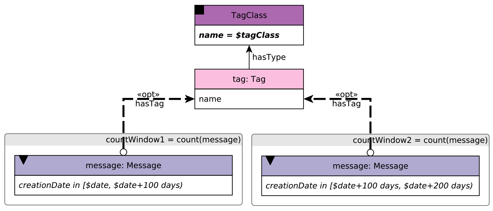
Figure 25. LDBC BI Query2.
This figure illustrates LDBC BI2 query. This query aims to find the Tags under a given TagClass that were used in Messages during in the 100-day time window starting at date and compare it with the 100-day time window that follows. For the Tags and for both time windows, compute the count of Messages.
The key to this query is creating two sub execution branches to count the two windows separately. We can use Gremlin’s by() step to achieve the purpose. Assume the TagClass's name='Actor' $date='2012-01-01', $date+100='2012-04-09'$ and $date+200='2012-07-18':
Firstly, we have to find all
Tagsrelated to the givenTagClassg.V().has("tagclass", "name", "Actor").in("hasType").as("tag")Then, we need to count for the first window: all the messages created from
2012-01-01to2012-04-09and having the specificTag. Since there are two separate counting tasks, we have to useselect()followed byby(...)step to create a new sub branch to execute the task..select("tag").by(__.in("hasTag").hasLabel("comment").has("creationDate", inside("2012-01-01", "2012-04-09")).dedup().count()).as("count1")Next, we need to count for the second window: all the messages created from
2012-04-09to2012-07-18and having the specificTag. Still, we useselect()followed byby(...)step to create a new sub branch to execute the task..select("tag").by(__.in("hasTag").hasLabel("comment").has("creationDate", inside("2012-04-09", "2012-07-18")).dedup().count()).as("count2")\Finally, we select
tag's name,count1andcount2from the traversers as the output.select("tag", "count1", "count2").by("name").by().by()')
Combine these procedures together, we can write the following code in GIE to make the LDBC BI2 query:
q1 = g.execute('g.V().has("tagclass", "name", "Actor").in("hasType").as("tag")\
                .select("tag").by(__.in("hasTag").hasLabel("comment")\
                .has("creationDate", inside("2012-01-01", "2012-04-09"))\
                .dedup().count()).as("count1")\
                .select("tag").by(__.in("hasTag").hasLabel("comment")\
                .has("creationDate", inside("2012-04-09", "2012-07-18"))\
                .dedup().count()).as("count2")\
                .select("tag", "count1", "count2")\
                .by("name").by().by()')
print(q1.all().result())
The output should be like:
# Query results for ldbc bi2 query
[{'count1': 0, 'count2': 0, 'tag': 'Jet_Li'},
 {'count1': 0, 'count2': 0, 'tag': 'Zhang_Yimou'},
 {'count1': 0, 'count2': 0, 'tag': 'Faye_Wong'},
 {'count1': 0, 'count2': 0, 'tag': 'Tsui_Hark'},
 {'count1': 3, 'count2': 7, 'tag': 'Bruce_Lee'},
 {'count1': 12, 'count2': 20, 'tag': 'Johnny_Depp'},
 {'count1': 6, 'count2': 4, 'tag': 'Tom_Cruise'},
 {'count1': 4, 'count2': 7, 'tag': 'Jackie_Chan'}]
LDBC BI3
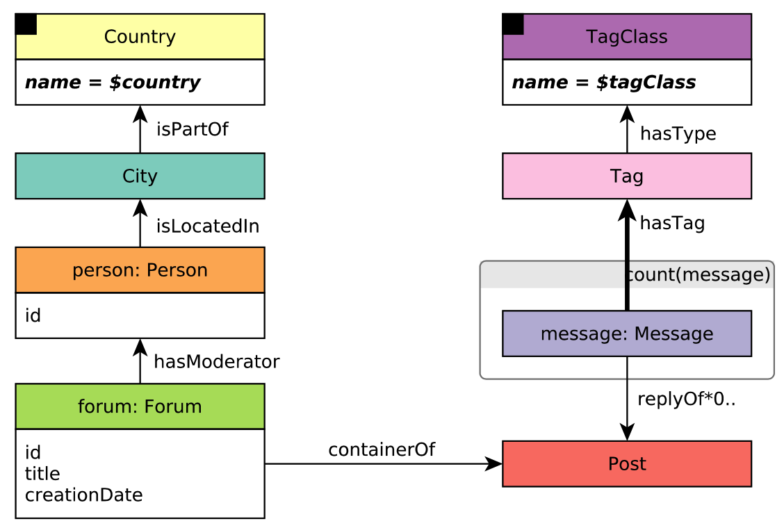
Figure 26. LDBC BI Query3.
This figure illustrates LDBC BI3 query. Given a TagClass and Country, this query aims to find all the Forums created in the given Country, containing at least one Message with Tags belonging directly to the given TagClass, and count the Messages by the Forum which contains them.
The location of a Forum is identified by the location of the Forum’s moderator. Here comes another question, how to determine whether the forum contains a message directly related to the given TagClass or not? We assume that a message is contained by a forum if:
It replies a post contained by the forum
It replies a message contained by the forum
Therefore, we can use out(1..) path expand step in Gremlin to find all the messages contained by a forum. However, the infinite path length may lead to serious computation cost. Therefore, the upper bound of the path expand is set to 6. Then we can use another two out('hasTag') and out('hasType') step followed by the filter has('name', TAGCLASS) to determine whether the message has required tag or not.
Assume the Country's name = 'China' and TagClass's name = 'Song', we can write in GIE as:
q1 = g.execute('g.V().has("place", "name", "China").in("isPartOf").in("isLocatedIn").as("person")\
            .in("hasModerator").as("forum").select("forum")\
            .by(out("containerOf").in("1..6", "replyOf").endV().as("message")\
            .out("hasTag").out("hasType").has("name", "Song")\
            .select("msg").dedup().count()).as("message_count")\
            .select("person", "forum", "message_count")\
            .by("id").by(valueMap("id", "title", "creationDate")).by())')
print(q1.all().result())
The output should be like:
# Query results for ldbc bi3 query
[{'forum': {'id': [824633725780],
   'creationDate': ['2012-01-08T02:52:34.334+0000'],
   'title': ['Album 3 of Hao Wang']},
  'person': 19791209300479,
  'message': 0},
 {'forum': {'id': [755914248304],
   'creationDate': ['2012-01-02T20:35:03.344+0000'],
   'title': ['Wall of Lin Lei']},
  'person': 24189255811275,
  'message': 0},
 {'forum': {'id': [824633725045],
   'creationDate': ['2012-02-03T18:15:52.633+0000'],
   'title': ['Album 4 of Lin Lei']},
  'person': 24189255811275,
  'message': 0},
 {'forum': {'id': [893353201782],
   'creationDate': ['2012-03-28T23:02:53.251+0000'],
   'title': ['Album 5 of Lin Lei']},
  'person': 24189255811275,
  'message': 0},
 {'forum': {'id': [1030792152809],
   'creationDate': ['2012-09-03T09:47:01.414+0000'],
   'title': ['Wall of Lei Chen']},
  'person': 32985348833887,
  'message': 0},
...
   'creationDate': ['2012-03-07T07:30:01.038+0000'],
   'title': ['Album 0 of Zhang Yang']},
  'person': 15393162789707,
  'message': 0},
 ...]
LDBC BI4(Left Part)
.png)
Figure 27. LDBC BI Query4(Left Part).
This figure illustrates the left part of the LDBC BI4 query. The query aims to find the top 100 forum of every country based on the memberCount, and the forum should be created after the given date.
Since GIE doesn’t provide global storage currently, we cannot pick out the top 100 forums of every country using Gremlin sentence directly. We can retrieve a tuple of (country, forum, country_count) at first.
Assume Forum's creationDate > '2012-01-01', we can write in GIE as
q1 = g.execute('g.V().hasLabel("place").as("country").in("isPartOf").in("isLocatedIn")\
           .in("hasMember").as("forum").dedup("country","forum")\
           .select("forum").by(out("hasMember").as("person").out("isLocatedIn")\
           .out("isPartOf").where(eq("country")).select("person").dedup().count())\
           .as("personCount").select("country", "forum", "personCount")')
print(q1.all().result())
The output should be like:
[{'forum': v[72057594037932503],
  'country': v[288230376151711797],
  'personCount': 2},
 {'forum': v[72057594037932473],
  'country': v[288230376151711797],
  'personCount': 1},
 {'forum': v[72057594037932489],
  'country': v[288230376151711797],
  'personCount': 1},
 {'forum': v[72057594037932494],
  'country': v[288230376151711797],
  'personCount': 1},
 {'forum': v[72057594037932501],
  'country': v[288230376151711797],
  'personCount': 2},
 {'forum': v[72057594037934803],
  'country': v[288230376151711797],
  'personCount': 1},
 {'forum': v[72057594037934804],
  'country': v[288230376151711797],
  'personCount': 1},
 {'forum': v[72057594037935005],
  'country': v[288230376151711797],
  'personCount': 2},
 {'forum': v[72057594037928132],
...
  'personCount': 1},
 {'forum': v[72057594037935879],
  'country': v[288230376151711799],
  'personCount': 1},
 ...]
Since GIE provides the python interface, then we can write codes to calculate the top 100 forum for each country very conveniently:
country_top100_forums_dict = {}
for traverser in q1.all().result():
    country = traverser['country']
    forum = traverser['forum']
    personCount = traverser['personCount']
    if country in country_top100_forums_dict:
        country_top100_forums_dict[country].append((forum, personCount))
    else:
        country_top100_forums_dict[country] = [(forum, personCount)]
for personCountForums in country_top100_forums_dict.values():
    personCountForums.sort(reverse=True, key=lambda x: x[1])
    if len(personCountForums) > 100:
        personCountForums = personCountForums[:100]
print(country_top100_forums_dict)
The result of LDBC BI Query 4(Left Part) should be like:
{v[288230376151711797]: [(v[72057594037935702], 7), (v[72057594037930685], 7), (v[72057594037932114], 6), (v[72057594037934231], 5), (v[72057594037935703], 5), (v[72057594037935730], 5), (v[72057594037935734], 5), (v[72057594037932509], 4), (v[72057594037935707], 4), (v[72057594037935708], 4), (v[72057594037935711], 4), (v[72057594037935714], 4), (v[72057594037935719], 4), (v[72057594037935729], 4), (v[72057594037935731], 4), (v[72057594037935724], 4), (v[72057594037929560], 4), (v[72057594037931546], 4), (v[72057594037931545], 4), (v[72057594037932479], 3), (v[72057594037932485], 3), (v[72057594037932505], 3), (v[72057594037932511], 3), (v[72057594037935710], 3), (v[72057594037935722], 3), (v[72057594037929246], 3), (v[72057594037928266], 3), (v[72057594037935713], 3), (v[72057594037934308], 3), (v[72057594037934313], 3), (v[72057594037934302], 3), (v[72057594037930430], 3), (v[72057594037934303], 3), (v[72057594037932503], 2), (v[72057594037932482], 2), (v[72057594037935147], 2), (v[72057594037935148], 2), (v[72057594037935157], 2), (v[72057594037927973], 2), (v[72057594037929386], 2), (v[72057594037934315], 2), (v[72057594037932501], 2), (v[72057594037935005], 2), (v[72057594037935720], 2), (v[72057594037935015], 2), (v[72057594037934300], 2), (v[72057594037930861], 2), (v[72057594037934319], 2), (v[72057594037931542], 2), (v[72057594037929583], 2), (v[72057594037933324], 2), (v[72057594037929182], 2), (v[72057594037929739], 2), (v[72057594037934829], 2), (v[72057594037935658], 2), (v[72057594037935660], 2), (v[72057594037935674], 2), (v[72057594037935682], 2), (v[72057594037935683], 2), (v[72057594037935672], 2), (v[72057594037927978], 2), (v[72057594037935163], 2), (v[72057594037935014], 2), (v[72057594037931544], 2), (v[72057594037934297], 2), (v[72057594037927979], 1), (v[72057594037932473], 1), (v[72057594037932474], 1), (v[72057594037934384], 1), (v[72057594037932639], 1), (v[72057594037934380], 1), (v[72057594037935146], 1), (v[72057594037935152], 1), (v[72057594037934804], 1), (v[72057594037928134], 1), (v[72057594037928674], 1), (v[72057594037929248], 1), (v[72057594037931240], 1), (v[72057594037931247], 1), (v[72057594037931256], 1), (v[72057594037930958], 1), (v[72057594037930963], 1), (v[72057594037931259], 1), (v[72057594037931260], 1), (v[72057594037931262], 1), (v[72057594037929365], 1), (v[72057594037929419], 1), (v[72057594037929421], 1), (v[72057594037929431], 1), (v[72057594037929434], 1), (v[72057594037929437], 1), (v[72057594037929446], 1), (v[72057594037929447], 1), (v[72057594037929449], 1), (v[72057594037929450], 1), (v[72057594037935166], 1), (v[72057594037929519], 1), (v[72057594037929451], 1), (v[72057594037929452], 1), (v[72057594037935046], 1), (v[72057594037932339], 1), (v[72057594037932481], 1), (v[72057594037934294], 1), (v[72057594037932389], 1), (v[72057594037932976], 1), (v[72057594037930870], 1), (v[72057594037931266], 1), (v[72057594037928092], 1), (v[72057594037928495], 1), (v[72057594037929510], 1), (v[72057594037929517], 1), (v[72057594037929961], 1), (v[72057594037929965], 1), (v[72057594037930242], 1), (v[72057594037930248], 1), (v[72057594037930250], 1), (v[72057594037930313], 1), (v[72057594037931547], 1), (v[72057594037935686], 1), (v[72057594037929052], 1), (v[72057594037929053], 1), (v[72057594037929055], 1), (v[72057594037929057], 1), (v[72057594037929060], 1), (v[72057594037934811], 1), (v[72057594037934813], 1), (v[72057594037934816], 1), (v[72057594037934821], 1), (v[72057594037934822], 1), (v[72057594037934823], 1), (v[72057594037934828], 1), (v[72057594037934835], 1), (v[72057594037934837], 1), (v[72057594037934975], 1), (v[72057594037934976], 1), (v[72057594037935032], 1), (v[72057594037935038], 1), (v[72057594037935045], 1), (v[72057594037935664], 1), (v[72057594037935673], 1), (v[72057594037935678], 1), (v[72057594037935685], 1), (v[72057594037931549], 1), (v[72057594037931550], 1), (v[72057594037931552], 1), (v[72057594037931554], 1), (v[72057594037931557], 1), (v[72057594037931560], 1), (v[72057594037931566], 1), (v[72057594037935671], 1), (v[72057594037935670], 1), (v[72057594037934977], 1), (v[72057594037931543], 1), (v[72057594037929518], 1), (v[72057594037935679], 1), (v[72057594037931575], 1), (v[72057594037932438], 1), (v[72057594037932878], 1), (v[72057594037932886], 1), (v[72057594037932888], 1), (v[72057594037927982], 1), (v[72057594037930526], 1), (v[72057594037930535], 1), (v[72057594037930546], 1), (v[72057594037930976], 1), (v[72057594037930536], 1), (v[72057594037931358], 1), (v[72057594037930366], 1), (v[72057594037931574], 1), (v[72057594037932435], 1), (v[72057594037935020], 1), (v[72057594037935864], 1), (v[72057594037933861], 1), (v[72057594037932440], 1), (v[72057594037927981], 1), (v[72057594037931349], 1), (v[72057594037931366], 1), (v[72057594037932885], 1), (v[72057594037927980], 1), (v[72057594037930529], 1), (v[72057594037930532], 1), (v[72057594037931304], 1), (v[72057594037932433], 1), (v[72057594037932441], 1), (v[72057594037934547], 1)], ......
LDBC BI11
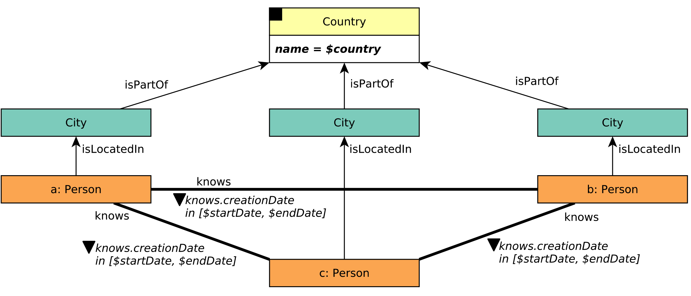
Figure 28. LDBC BI Query11.
This figure illustrates LDBC BI11 query. This query aims to find three persons tagged as a, b, c, where:
a, b, c know each other
a, b, c live in the same country
their relationship(‘knows’) were created in the range [
startDate,endDate]
It is easy to use Gremlin’s match(...) step to describe this query. Assume the Country's name=China, the startDate='2012-01-01', the endDate='2012-07-01':
q1 = g.execute('g.V().match(__.as("a").bothE("knows")\
                              .has("creationDate", inside("2012-01-01", "2012-07-01"))\
                              .otherV().as("b"),\
                            __.as("a").bothE("knows")\
                              .has("creationDate", inside("2012-01-01", "2012-07-01"))\
                              .otherV().as("c"),\
                            __.as("a").bothE("knows")\
                               .has("creationDate", inside("2012-01-01", "2012-07-01"))\
                               .otherV().as("c"),\
                            __.as("a").out("isLocatedIn").out("isPartOf").as("d"),\
                            __.as("b").out("isLocatedIn").out("isPartOf").as("d"),\
                            __.as("c").out("isLocatedIn").out("isPartOf").as("d"),\
                            __.as("d").has("name", "China").as("d"))\
                     .select("a", "b", "c")')
print(q1.all().result())
The output should be like:
# Query results for ldbc bi11 query
[{'a': v[216172782113784091], 'b': v[216172782113783882], 'c': v[216172782113784250]}, ......,
 {'a': v[216172782113784403], 'b': v[216172782113784537], 'c': v[216172782113784122]}]
LDBC BI14
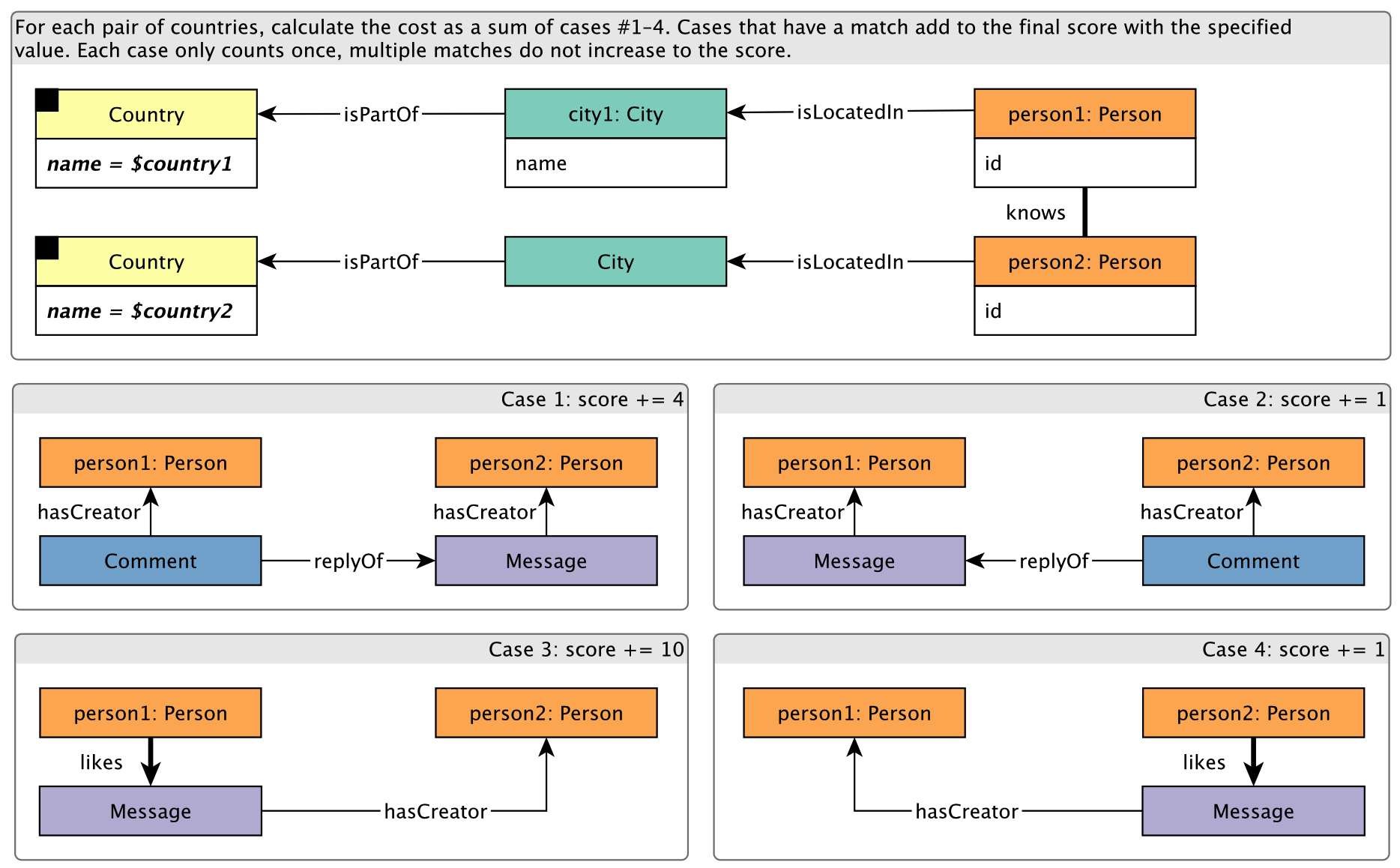
Figure 29. LDBC BI Query14.
This figure illustrates LDBC BI14 query. Here is its purpose:
Consider all pairs of people (person1, person2) such that
they know each other,
one is located in a City of Country
country1,and the other is located in a City of Country
country2.
For each City of Country country1, return the highest scoring pair. The score of a pair is defined as the sum of the subscores awarded for the following kinds of interaction. The initial value is score = 0.
person1has created a replyCommentto at least oneMessagebyperson2: score += 4person1has created at least oneMessagethatperson2has created a reply to: score += 1person1liked at least oneMessagebyperson2: score += 10person1has created at least oneMessagethat was liked byperson2: score += 1
Assume country1's name = "India" and country2's name = "Chile", we can write in GIE as:
q1 = g.execute('g.V().has("place", "name", "India")\
                .in("isPartOf").in("isLocatedIn").as("p1")\
                .both("knows").as("p2").out("isLocatedIn").out("isPartOf")\
                .has("name", "Chile")\
                .select("p1").by(in("hasCreator").hasLabel("comment").out("replyOf")\
                .out("hasCreator").where(eq("p2")).select("p1").dedup().count()).as("case1")\
                .select("p1").by(in("hasCreator").in("replyOf").hasLabel("comment")\
                .out("hasCreator").where(eq("p2")).select("p1").dedup().count()).as("case2")\
                .select("p1").by(out("likes").hasLabel("post", "comment")\.out("hasCreator")\\
                .where(eq("p2"))\.select("p1").dedup().count()).as("case3")\
                .select("p1").by(in("hasCreator").hasLabel("post", "comment").in("likes")\
                .where(eq("p2")).select("p1").dedup().count()).as("case4")\
                .select(expr("@case1 * 4 + @case2 * 1 + @case3 * 10 + @case4 * 1")).as("score")\
                .select("p1", "p2", "score")')
print(q1.all().result())
The output of LDBC BI14 query should be like:
# Query results for ldbc bi14 query
[{'p1': v[216172782113784153], 'score': 10, 'p2': v[216172782113784100]},
 {'p1': v[216172782113783956], 'score': 10, 'p2': v[216172782113784673]},
 {'p1': v[216172782113784252], 'score': 10, 'p2': v[216172782113784263]},
 {'p1': v[216172782113784193], 'score': 0, 'p2': v[216172782113784100]},
 {'p1': v[216172782113784242], 'score': 6, 'p2': v[216172782113784263]},
 {'p1': v[216172782113784623], 'score': 11, 'p2': v[216172782113784498]},
 {'p1': v[216172782113784251], 'score': 5, 'p2': v[216172782113784538]},
 {'p1': v[216172782113784167], 'score': 11, 'p2': v[216172782113784100]},
 {'p1': v[216172782113783864], 'score': 12, 'p2': v[216172782113784100]},
 {'p1': v[216172782113784613], 'score': 5, 'p2': v[216172782113784116]},
 {'p1': v[216172782113784481], 'score': 16, 'p2': v[216172782113784498]},
 {'p1': v[216172782113784481], 'score': 16, 'p2': v[216172782113784100]}]