Graph Learning Workloads
What is Graph Neural Network
Graph neural networks (GNNs) are a type of neural network designed to work with graph data structures, consisting of nodes and edges. GNNs learn to represent each node in the graph by aggregating information from its neighboring nodes in multiple hops, which allows the model to capture complex relationships between nodes in the graph. This involves a process of message passing between nodes, where each node receives messages from its neighboring nodes and updates its representation based on the aggregated information. By iteratively performing this process, GNNs can learn to capture not only the local features of a node but also its global position in the graph, making them particularly useful for tasks such as node classification, link prediction, and graph classification.
Node classification is a task (GNNs) where the goal is to predict the label of each node in a graph. In other words, given a graph with nodes and edges, the task is to assign a category or class to each node based on the features of the node and its connections to other nodes. This is an important task in many applications such as social network analysis and drug discovery. GNNs are particularly suited for node classification as they can capture the structural information and relationships between nodes in a graph, which can be used to improve the accuracy of the classification.
Link prediction is a key task in GNNs that aims to predict the existence or likelihood of a link between two nodes in a graph. This task is important in various applications, such as recommendation systems and biology network analysis, where predicting the relationships between nodes can provide valuable insights. GNNs can effectively capture the structural information and features of the nodes to improve the accuracy of link prediction. The task is typically framed as a binary classification problem where the model predicts the probability of a link existing between two nodes.
Graph classification is another GNN task that aims to classify an entire graph into one or more classes based on its structure and features. This task is used in various domains, such as bioinformatics, social network analysis, and chemical structure analysis. The task is typically framed as a multi-class classification problem where the model predicts the probability of the graph belonging to each class. GNNs have shown promising results in graph classification tasks and have outperformed traditional machine learning models.
The learning engine in GraphScope (GLE) is driven by Graph-Learn, a distributed framework designed for development and training of large-scale graph neural networks (GNNs). GLE provides a programming interface carefully designed for the development of graph neural network models, and has been widely applied in many scenarios within Alibaba, such as search recommendation, network security and knowledge graphs.
Typical GNN Models
First, let’s briefly rewind the concept of GNN. Given a graph \(G = (V,E)\), where each vertex is associated with a vector of data as its feature. Graph Neural Networks(GNNs) learn a low-dimensional embedding for each target vertex by stacking multiple GNNs layers \(L\). For each layer, every vertex updates its activation by aggregating features or hidden activations of its neighbors \(N(v),v \in V\).
There are several types of GNN models used for various tasks, such as node classification, link prediction, and graph classification. Here are some of the most common types of GNN models:
Graph Convolutional Networks (GCN): GCN is a popular GNN model used for node classification and graph classification tasks. It applies a series of convolutional operations to the graph structure, allowing the model to learn representations of nodes and their neighborhoods.
Graph Attention Networks (GAT): GAT is another popular GNN model that uses attention mechanisms to weigh the importance of neighboring nodes when computing node representations. It has been shown to outperform GCN on several benchmark datasets.
GraphSAGE: GraphSAGE is a variant of GCN that uses a neighborhood aggregation strategy to generate node embeddings. It allows the model to capture high-order neighborhood information and scalable to large graphs.
There are also many other types of GNN models, such as Graph Isomorphism Networks (GIN), Relational Graph Convolutional Network (R-GCN), and many more. The choice of GNN model depends on the specific task and the characteristics of the input graph data.
Paradigm of Model Training
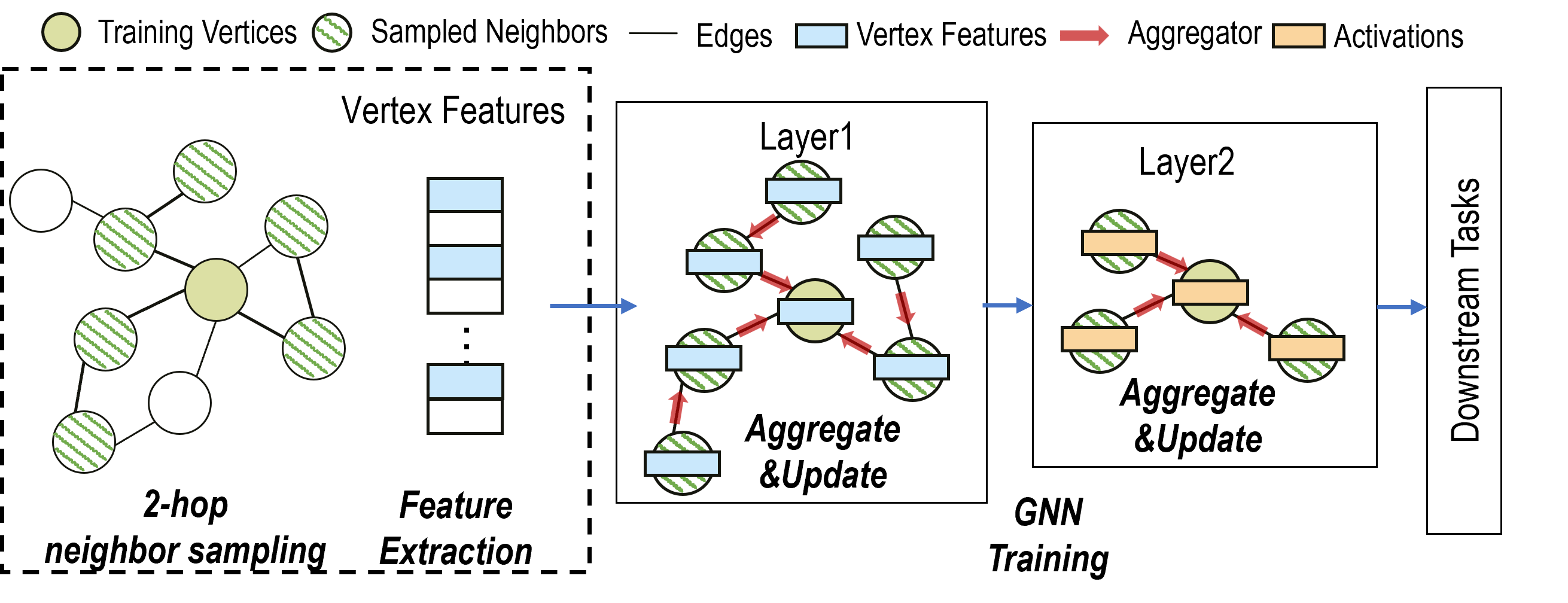
In general, there are two ways to train a GNN model: (1) whole graph training and (2) mini-batch training. Whole graph training is to compute based on the whole graph directly. The GCN and GAT are originally proposed using this approach, directly computing on the entire adjacency matrix. However, this approach will consume huge amount of memory on large-scale graphs, limiting its applicability. Mini-batch training is a practical solution for scaling GNN training on very large graphs. Neighbor sampling is used to generate mini-batches, allowing sampling-based GNN models to handle unseen vertices. GraphSAGE is a typical example of mini-batch training. The following figure illustrates the workflow of 2-hop GraphSAGE training.
Steps of Model Training
The process of training a GNN involves several steps, which are described below.
Data Preparation: The first step in training a GNN is to prepare the input data. This involves creating a graph representation of the data, where nodes represent entities and edges represent the relationships between them. The graph can be represented using an adjacency matrix or an edge list. The features of the original graph data may be complex and cannot be directly accessed for model training. For example, the node features “id=123456, age=28, city=Beijing” and other plain texts need to be processed into continuous features by embedding lookup. The type, value space, and dimension of each feature after vectorization should be clearly described when adding vertex or edge data sources.
Model Initialization: After the data is prepared, the next step is to initialize the GNN model. This involves selecting an appropriate architecture for the model and setting the initial values of the model parameters.
Forward and Backward Pass: During the forward pass, the GNN model takes the input graph(sampled subgraphs in mini-batch training) and propagates information through the graph, updating the embedding of each node based on the embedding of its neighbors. The difference between the predicted output and the ground truth is measured by the loss function. In the backward pass, the gradients of the loss function with respect to the model parameters are computed, and are used to update the model parameters.
Iteration: Step 3 is repeated iteratively until the model converges to a satisfactory level of performance. During each iteration, the model parameters are updated based on the gradients of the loss function, and the quality of the model prediction is evaluated using a validation set.
Evaluation: After the model is trained, it is evaluated using a test set of data to measure its performance on unseen data. Various evaluation metrics such as accuracy, precision, recall, and F1 score can be used to assess the performance of the model.
Subgraph Sampling
In practical industrial applications, the size of
the graph is often relatively large and the features on the nodes and edges of the graph
are complex (there may be both discrete and continuous features). Thus it is not possible
to perform message passing/neighbor aggregation directly on the original graph. A feasible
and efficient approach is based on the idea of graph sampling, where a subgraph is first
sampled from the original graph and then the computation is based on the subgraph.
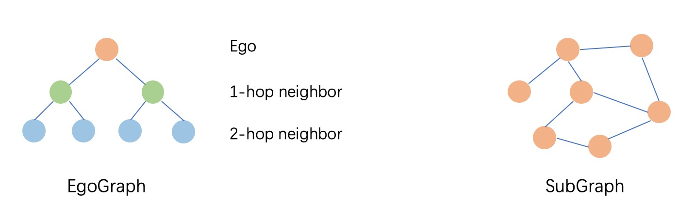
According to the difference of neighbor sampling operator in subgraph sampling and
NN operator in message passing, we organize the subgraph into EgoGraph or SubGraph
format. EgoGraph consists of the central object ego and its fixed-size neighbors, which
is a dense organization format. SubGraph is a more general subgraph organization format,
consisting of nodes, edges features and edge index (a two-dimensional array consisting
of row index and column index of edges), generally using full neighbor. The conv layer
based on SubGraph generally uses the sparse NN operator. The examples of EgoGraph and
SubGraph are shown in the following figure.
Challenges of Applying GNNs on Large Graphs
Based on our experience, applying GNN to industrial-scale large graphs requires addressing the following challenges:
Data irregularity: One of the challenges of GNN is to handle various forms of unstructured data, such as sparse, directed, undirected, homogeneous, and heterogeneous data, as well as node and edge attributes. These data types may require different graph processing methods and algorithms.
Scalability: In industrial scenarios, graph data is usually very large, containing a large number of nodes and edges. This leads to problems with computation and storage, as well as the problem of exponential data expansion through sampling.
Computational complexity: GNN has a very high computational complexity because it requires the execution of multiple operators, including graph convolution, pooling, activation, etc. These operators require efficient algorithms and hardware support to enable GNN to run quickly on large-scale graphs.
Dynamic graph: In industrial scenarios, the graph structure and attributes may undergo real-time changes, which may cause GNN models to fail to perceive and adapt to these changes in time.
Overall, the application of GNN in industrial scenarios has many challenges and requires research and optimization of algorithms, computation, storage, and data, etc., in order to better meet practical application needs.
What can GraphScope Do
In GraphScope, Graph Learning Engine (GLE) addresses the aforementioned challenges in the following ways:
Managing graph data in a distributed way
In GraphScope, graph data is represented as property graph model. To support large-scale graph, GraphScope automatically partitions the whole graph into several subgraphs (fragments) distributed into multiple machines in a cluster. Meanwhile, GraphScope provides user-friendly interfaces for loading graphs to allow users to manage graph data easily. More details about how to manage large-scale graphs can refer to this. GLE performs graph-related computations, such as distributed graph sampling and feature collection, on this distributed graph storage.
Built-in GNN models and PyG compatible
GLE comes with a rich set of built-in GNN models, like GCN, GAT, GraphSAGE, and SEAL, and provides a set of paradigms and processes to ease the development of customized models. GLE is compatible with PyG, e.g., this example shows that a PyG model can be trained using GLE with very minor modifications. Users can flexibly choose TensorFlow or PyTorch as the training backend.
Inference on dynamic graph
To support online inference on dynamic graphs, we propose Dynamic Graph Service (DGS) in GLE to facilitate real-time sampling on dynamic graphs. The sampled subgraph can be fed into the serving modules (e.g., TensorFlow Serving) to obtain the inference results. This document is organized to provide a detailed, step-by-step tutorial specifically demonstrating the use of GLE for offline training and online inference.