A Review of Programming Models for Parallel Graph Processing
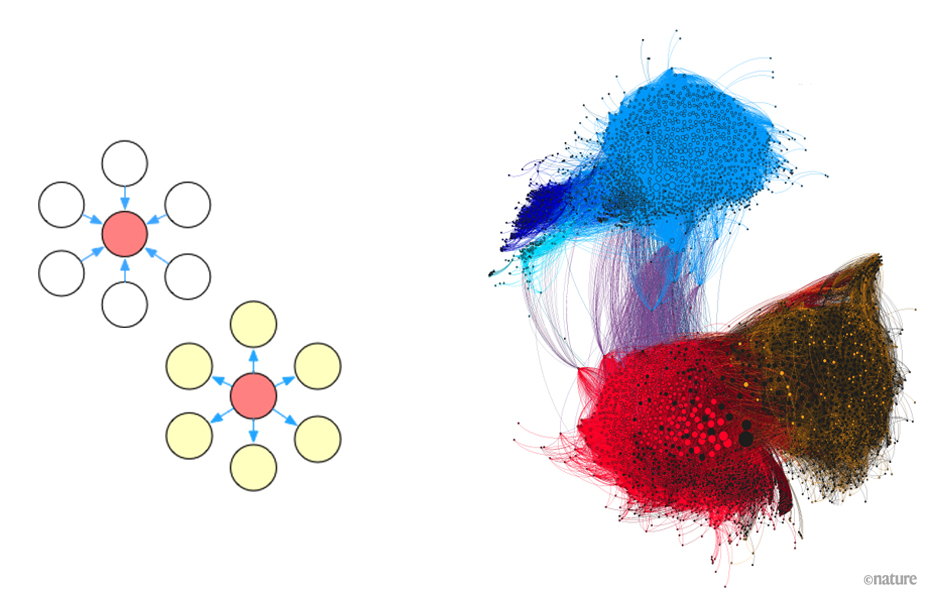 To explore underlying insights hidden in graph data, many graph analytics algorithms, e.g., PageRank and single source shortest paths (the Dijkstra’s algorithm), have been designed to solve different problems.
In a single machine environment, developers can easily implement sequential solutions to these algorithms as they have a global view of the graph and can freely iterate through all vertices and edges. Current graph data in real industrial scenarios usually consists of billions of vertices and trillions of edges. Such a graph has to be divided into multiple partitions, and stored and processed in a distributed/parallel way. To allow developers to succinctly express graph algorithms under such environment, many programming models for parallel graph processing have been proposed. In this post, we would like to introduce some commonly used programming models, and further discuss their pros and cons.
Think like a vertex
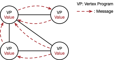
The vertex-centric model proposed in Pregel[1] follows the philosophy of “think like a vertex”, where each vertex contains information about itself as well as all its adjacent edges, and the computation is expressed at the level of a single vertex. More specifically, the entire computation process is divided into multiple iterations (called supersteps), and in each superstep, all vertices execute the same user-defined function (called vertex program) that expresses the logic of a given algorithm. The vertex program defines how each vertex processes incoming messages (sent in the previous superstep), and sends messages to other vertices (for the next superstep). The iterations terminate until no messages are sent from any vertex, indicating a halt.
With the vertex-centric model, the vertex program of single source shortest paths (SSSP) is expressed as follows.
def VertexProgramForSSSP():
    # receive and merge incoming messages
    incoming_msgs = ReceiveMessages()
    merged_msg = Reduce(incoming_msgs, MIN)

    # update vertex property
    if dist > merged_msg:
        dist = merged_msg

    # send messages to neighbors
    for neighbor in neighbors:
        if dist + edge_weight < neighbor_dist:
            SendMessage(neighbor, dist + edge_weight)
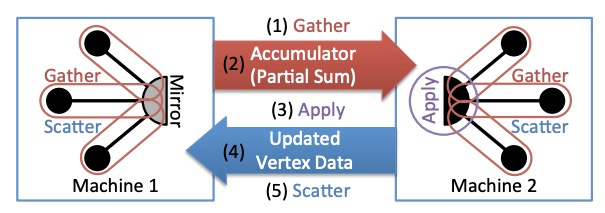
However, the performance of Pregel drops dramatically when facing natural graphs which follow a power-law distribution. To solve this problem, PowerGraph[2] proposed the GAS (Gather-Apply-Scatter) programming model for the vertex-cut graph partitioning strategy. The Gather function runs locally on each partition and then one accumulator is sent from each mirror to the master. The master runs the Apply function and then sends the updated vertex data to all mirrors. Finally, the Scatter phase is run in parallel on mirrors to update the data on adjacent edges.
Following the GAS abstraction, the SSSP can be implemented as follows.
def GASForSSSP():
    # gather_nbrs: ALL_NBRS
    def gather(D_u, D(u,v), D_v):
        return D_v + D(v,u)

    def sum(a, b):
        return min(a, b)

    def apply(D_u, new_dist):
        D_u = new_dist

    # scatter_nbrs: ALL_NBRS
    def scatter(D_u,D(u,v),D_v):
        # If changed, activate neighbor
	if(changed(D_u)):
	    Activate(v)
	if(increased(D_u)):
	    return NULL
	else:
            return D_u + D(u,v)
Pros:
- Powerful expressiveness to express various graph algorithms.
- The vertex program is easy to run parallelly.
Cons:
- Existing sequential (single-machine) graph algorithms have to be modified to comply with the “think like a vertex” principle.
- Each vertex is very short-sighted: it only has information about its 1-hop neighbors, and thus information is propagated through the graph slowly, one hop at a time. As a result, it may take many computation iterations to propagate a piece of information from a source to a destination.
Think like a graph
To tackle the problem of short-sighted vertices in the vertex-centric model, the subgraph-centric (a.k.a. block-centric, partition-centric) programming model[3, 4] is proposed. Different from the vertex-centric model, the subgraph-centric model focuses on the entire subgraph, and is labeled as “think like a graph”. For the vertex-centric model, it uses the information of 1-hop neighbors to update the value of each vertex in one superstep. Instead, the subgraph-centric model leverages information within the whole subgraph. In addition, each vertex can send messages to any vertex in the graph, instead of 1-hop neighbors. In this way, the communication overhead and the number of supersteps are greatly reduced.
The SSSP is expressed as follows in the subgraph-centric model.
def ComputeSSSP(subgraph, messages):
    # vertices with improved distances
    openset = NULL
    if superstep == 1: # initialize distances
    	for v in subgraph.internal_vertices:
	    if v == SOURCE:
		v.value = 0 # set distance to source as 0
		openset.add(v) # distance has improved
	    else:
		v.value = MAX_INT # not source vertex
	for m in messages: # process input messages
	    if subgraph.vertices[m.vertex].value > m.value:
		subgraph.vertices[m.vertex].value = m.value
		openset.add(m.vertex) # distance improved
	boundarySet = dijkstra(openset)
	# Send new distances to boundary vertices
	for (boundarySG, vertex, value) in boundarySet:
	    SendToSubgraphVertex(boundarySG, vertex, value)
	VoteToHalt()

def dijkstra(openset):
    boundaryOpenset = NULL
    while openset is not NULL:
	v = GetShortestVertex(openset)
	for v2 in v.neighbors:
            # update neighbors, notify if boundary.
	    if v2.isBoundary():
		boundaryOpenset.add(v2.subgraph,v2,v.value+dis(v,v2))
	    else if v2.value > v.value + dis(v,v2):
		v2.value = v.value + dis(v,v2)
		openset.add(v2) # distance has improved
	openset.remove(v) # done with this local vertex
    return boundaryOpenset
Pros:
- The same expressiveness with the vertex-centric model.
- Offer lower communication overhead, lower scheduling overhead, and lower memory overhead compared with vertex-centric approaches.
Cons:
- Still need to recast existing sequential graph algorithms into the new programming model.
- Developers need to know a lot of concepts (e.g., internal and boundary vertices), causing the implementation challenge.
Think sequential, run parallel
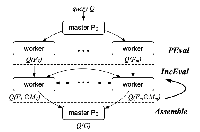
To make parallel graph computations accessible to average users while achieving high performance at the same time, the PIE (PEval-IncEval-Assemble) programming model[5] is proposed. In this model, users only need to provide three functions,
- (1) PEval, a sequential (single-machine) function for given a query, computes the answer on a local partition;
- (2) IncEval, a sequential incremental function, computes changes to the old output by treating incoming messages as updates; and
- (3) Assemble, which collects partial answers, and combines them into a complete answer.
The PIE model works on a graph G and each worker maintains a partition of G. Given a query, each worker first executes PEval against its local partition, to compute partial answers in parallel. Then each worker may exchange partial results with other workers via synchronous message passing. Upon receiving messages, each worker incrementally computes IncEval. The incremental step iterates until no further messages can be generated. At this point, Assemble pulls partial answers and assembles the final result. In this way, the PIE model parallelizes existing sequential graph algorithms, without revising their logic and workflow.
The following pseudo-code shows how SSSP is expressed in the PIE model, where the Dijkstra’s algorithm is directly used for the computation of parallel SSSP.
def dijkstra(g, vals, updates):
    heap = VertexHeap()
    for i in updates:
	vals[i] = updates[i]
	heap.push(i, vals[i])

    updates.clear()

    while not heap.empty():
	u = heap.top().vid
	distu = heap.top().val
	heap.pop()
	for e in g.get_outgoing_edges(u):
	    v = e.get_neighbor()
	    distv = distu + e.data()
	    if vals[v] > distv:
		vals[v] = distv
		    if g.is_inner_vertex(v):
			heap.push(v, distv)
			updates[v] = distv
	return updates

def PEval(source, g, vals, updates):
    for v in vertices:
        updates[v] = MAX_INT
    updates[source] = 0
    dijkstra(g, vals, updates)

def IncEval(source, g, vals, updates):
    dijkstra(g, vals, updates)
Currently, the PIE model has been developed and evaluated in the graph analytical engine of GraphScope. On the LDBC Graph Analytics benchmark, GraphScope outperforms other state-of-the-art graph processing systems (see link). Welcome to try and develop your own graph algorithms with GraphScope.
References
- Some images in this article are cited from [2] and https://twitter.com/katestarbird/status/1358088750765539329/photo/1.
- [1] Malewicz, Grzegorz, et al. “Pregel: a system for large-scale graph processing.” Proceedings of the 2010 ACM SIGMOD International Conference on Management of data. 2010.
- [2] Gonzalez, Joseph E., et al. “Powergraph: Distributed graph-parallel computation on natural graphs.” 10th USENIX Symposium on Operating Systems Design and Implementation (OSDI 12). 2012.
- [3] Tian, Yuanyuan, et al. “From” think like a vertex” to” think like a graph”.” Proceedings of the VLDB Endowment 7.3 (2013): 193-204.
- [4] Yan, Da, et al. “Blogel: A block-centric framework for distributed computation on real-world graphs.” Proceedings of the VLDB Endowment 7.14 (2014): 1981-1992.
- [5] Fan, Wenfei, et al. “Parallelizing sequential graph computations.” ACM Transactions on Database Systems (TODS) 43.4 (2018): 1-39.