Analyzing Graphs with GraphScope in the Style of NetworkX
 This article demonstrate how to analyze graph with GraphScope in the style of NetworkX.
NetworkX is a tool for graph theory and complex network modeling developed in Python
and it has a simple and easy-to-use graph analysis interface. GraphScope provides a set of NetworkX-compatible graph analysis interfaces that not only support the use of simple and easy-to-use interfaces like NetworkX but also provide high-performance graph analysis algorithms to support the processing of ultra-large-scale graph data.
This article demonstrate how to analyze graph with GraphScope in the style of NetworkX.
NetworkX is a tool for graph theory and complex network modeling developed in Python
and it has a simple and easy-to-use graph analysis interface. GraphScope provides a set of NetworkX-compatible graph analysis interfaces that not only support the use of simple and easy-to-use interfaces like NetworkX but also provide high-performance graph analysis algorithms to support the processing of ultra-large-scale graph data.
What is NetworkX
NetworkX is a tool for graph theory and complex network modeling developed in Python. It comes with built-in graph and complex network analysis algorithms and provides a simple and easy-to-use graph analysis interface that allows for easy analysis of complex network data and simulation modeling. NetworkX’s interface design is very concise, making it easy for novices to quickly develop their understanding of graph data. Furthermore, the interface is easy to use for small to medium-sized data sets.
However, because NetworkX is based on the Python language, algorithm performance is not its strong suit, and it cannot effectively handle industrial-level large-scale graph data. In response to this challenge, GraphScope provides a set of NetworkX-compatible graph analysis interfaces that not only support the use of simple and easy-to-use interfaces like NetworkX but also provide high-performance graph analysis algorithms to support the processing of ultra-large-scale graph data.
We will use a small example to briefly introduce the graph analysis process of NetworkX.
import networkx

# initialize an empty undirected graph
G = networkx.Graph()

# add edge lists through the "add_edges_from" interface.
# here we add two edges (1, 2) and (1, 3)
G.add_edges_from([(1, 2), (1, 3)])

# add node 4 through the "add_node" interface
G.add_node(4)

# check some graph information
# use "G.number_of_nodes()" to query the current number of nodes/vertices in graph G
G.number_of_nodes()
# 4

# similarly, "G.number_of_edges()" can query the number of edges in graph G
G.number_of_edges()
# 2

# use "G.degree" to query the degree of each vertex in graph G
sorted(d for n, d in G.degree())
# [0, 1, 1, 2]

# finally, call the built-in algorithm of NetworkX to analyze the graph
# here we call the "connected_components" algorithm to analyze the connected components of graph G
list(networkx.connected_components(G))
# [{1, 2, 3}, {4},]

# and call the "clustering" algorithm to analyze the clustering of graph G
networkx.clustering(G)
# {1: 0, 2: 0, 3: 0, 4: 0}
The above example is just a simple introduction to graph analysis with NetworkX. For more information on NetworkX interfaces, detailed usage instructions, and built-in algorithms, please refer to the official NetworkX documentation.
Analysis with GraphScope in the Style of NetworkX
The official NetworkX tutorial is a beginner’s guide to using the NetworkX interface and graph analysis. To demonstrate GraphScope’s compatibility with NetworkX and how to use GraphScope’s NetworkX interface for graph analysis, we will use GraphScope to execute the examples in the tutorial.
Using GraphScope’s NetworkX compatible interface, we simply replace import networkx as nx with import graphscope.nx as nx to use the same conventions as NetworkX.
Of course, we can use other custom aliases, such as import graphscope.nx as gs_nx.
Creating a Graph
GraphScope supports the same graph syntax as NetworkX. In the example, we use nx.Graph() to create an empty undirected graph.
import graphscope.nx as nx

# initialize an empty undirected graph
G = nx.Graph()
Adding Nodes and Edges
GraphScope’s graph operation functions are also compatible with NetworkX. Users can add nodes through
add_node and add_nodes_from and add edges through add_edge and add_edges_from.
# add a node with "add_node"
G.add_node(1)

# or add nodes from any iterable container, such as a list
G.add_nodes_from([2, 3])

# if the container is in the form of a tuple, you can also add node attributes while adding nodes
G.add_nodes_from([(4, {"color": "red"}), (5, {"color": "green"})])

# for edges, you can add one edge with "add_edge"
G.add_edge(1, 2)
e = (2, 3)
G.add_edge(*e)

# add edge lists with "add_edges_from"
G.add_edges_from([(1, 2), (1, 3)])

# or add edge attributes while adding edges through edge tuples
G.add_edges_from([(1, 2), (2, 3, {'weight': 3.1415})])
Querying Graph Elements
GraphScope supports NetworkX-compatible graph query interfaces. Users can use number_of_nodes and
number_of_edges to obtain the number of nodes and edges in the graph, and use nodes, edges,
adj, and degree interfaces to obtain the current nodes and edges in the graph, as well as
information such as node neighbors and degrees.
# query the current number of nodes and edges in the graph
G.number_of_nodes()
# 5
G.number_of_edges()
# 3

# list the nodes and edges currently in the graph
list(G.nodes)
# [1, 2, 3, 4, 5]
list(G.edges)
# [(1, 2), (1, 3), (2, 3)]

# query the neighbors of a node
list(G.adj[1])
# [2, 3]

# query the degree of a node
G.degree(1)
# 2
Removing Elements from the Graph
Like NetworkX, GraphScope can also modify the graph by removing nodes and edges from the graph in a way
similar to adding elements. For example, you can use remove_node and remove_nodes_from to delete
nodes from the graph, and remove_edge and remove_edges_from to delete edges from the graph.
# remove a node with "remove_node"
G.remove_node(5)

# check the nodes in graph, and we can see that node 5 has been removed
list(G.nodes)
# [1, 2, 3, 4]

# remove multiple nodes using "remove_nodes_from"
G.remove_nodes_from([4, 5])

# check the nodes in graph G, and we can see that node 4 has also been removed
list(G.nodes)
# [1, 2, 3]

# remove an edge using "remove_edge"
G.remove_edge(1, 2)

# check the edges in graph G now, and we can see that edge (1, 2) has been removed
list(G.edges)
# [(1, 3), (2, 3)]

# remove multiple edges using "remove_edges_from"
G.remove_edges_from([(1, 3), (2, 3)])

# check the edges in graph G now, and we can see that edges (1, 3) and (2, 3) no longer exist in G
list(G.edges)
# []

# let's check the number of nodes and edges now
G.number_of_nodes()
# 3

G.number_of_edges()
# 0
Analyzing Graph
GraphScope can perform various graph analysis algorithms through its NetworkX-compatible interface.
In the example, we build a simple graph and use connected_components algorithm to analyze the graph’s connected components,
use clustering algorithm to obtain the clustering coefficients of each point in the graph,
and use all_pairs_shortest_path algorithm to obtain the shortest path between nodes.
# first create the graph
G = nx.Graph()
G.add_edges_from([(1, 2), (1, 3)])
G.add_node(4)

# use the connected_components algorithm to find the connected components in the graph
list(nx.connected_components(G))
# [{4}, {1, 2, 3},]

# use the clustering algorithm to calculate the clustering coefficient of each node
nx.clustering(G)
# {4: 0.0, 1: 0.0, 2: 0.0, 3: 0.0}

# calculate the shortest path between each pair of nodes in the graph
sp = dict(nx.all_pairs_shortest_path(G))

# check the shortest path between node 3 and other nodes
sp[3]
# {3: [3], 1: [3, 1], 2: [3, 1, 2]}
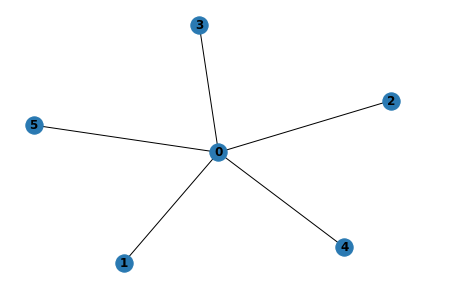
Drawing Graph
Like NetworkX, GraphScope supports simple graph drawing through draw.
import graphscope.nx as nx

# create a star graph with 5 nodes
G = nx.star_graph(5)

# draw the graph with "nx.draw"
nx.draw(G, with_labels=True)
Through some simple examples, we have shown the compatibility of GraphScope with the NetworkX interface and demonstrated the use of some graph operation/analysis interfaces. More detailed usage can be found in the GraphScope documentation.
Magnitude of Performance Improvement compared to NetworkX
GraphScope supports some of the built-in graph algorithms in NetworkX, and we can call these algorithms by calling the NetworkX algorithm. Below, we use a simple experiment to see how much GraphScope improves algorithm performance compared to NetworkX.
This experiment uses twitter data from SNAP, and tests the Clustering algorithm built into NetworkX. The machine used for the experiment has 8 CPUs and 16G of memory.
First, we prepare the data and use wget to download the dataset to the local environment.
wget https://raw.githubusercontent.com/GraphScope/gstest/master/twitter.e ${HOME}/twitter.e
Then we load the snap-twitter data into GraphScope and NetworkX separately.
import os
import graphscope.nx as gs_nx
import networkx as nx

# load snap-twitter data into NetworkX
g1 = nx.read_edgelist(
     os.path.expandvars('$HOME/twitter.e'),
     nodetype=int,
     data=False,
     create_using=nx.Graph
)
type(g1)
# networkx.classes.graph.Graph

# load snap-twitter data into GraphScope
g2 = gs_nx.read_edgelist(
     os.path.expandvars('$HOME/twitter.e'),
     nodetype=int,
     data=False,
     create_using=gs_nx.Graph
)
type(g2)
# graphscope.nx.classes.graph.Graph
We use the Clustering algorithm to analyze the graph and see how much GraphScope improves algorithm performance compared to NetworkX.
%%time
# calculate the clustering coefficient of each node in the graph using GraphScope
ret_gs = gs_nx.clustering(g2)
# CPU times: user 213 ms, sys: 163 ms, total: 376 ms
# Wall time: 2.9 s

%%time
# calculate the clustering coefficient of each node in the graph using NetworkX
ret_nx = nx.clustering(g1)
# CPU times: user 54.8 s, sys: 0 ns, total: 54.8 s
# Wall time: 54.8 s

# compare the results
ret_gs == ret_nx
# True
From the experimental results, we can see that GraphScope’s built-in algorithms can achieve several orders of magnitude performance improvement compared to NetworkX, while providing simple and easy-to-use interfaces compatible with NetworkX.
Conclusion
This article introduces how to use GraphScope to operate and analyze graph in the style of NetworkX. Furthermore, we compare GraphScope’s compatibility with NetworkX interfaces and its high-performance analytical capabilities using clustering algorithms analyzed on the snap-twitter graph data.