Simplifying Complex Graph Loading with Jupyter Notebook
 Schema construction and graph data loading are usually the complicated steps in graph computing processes. Currently, GraphScope has released a graphscope-notebook plugin which through an interactive way help users complete the graph loading in the Jupyterlab environment. This article will provide a detailed introduction to the use of this plugin, and users can try it in the Playground environment.
Background
For any graph computing product, the loading of graph data is often the first and most important step, as well as a very complicated step, mainly due to the complexity of the graph data itself. Therefore, in order to improve the loading experience, GraphScope has built-in various datasets. For example, for the TinkerPop Modern Graph, users just need one statement to complete the loading operation:
>>> from graphscope.dataset import load_modern_graph
>>> modern_graph = load_modern_graph()
However, for the user’s dataset, the loading process needs to define a very long code, we use ogbn-mag this property graph as an example:
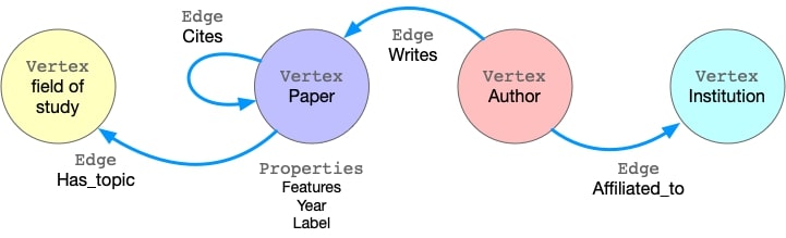
This graph has four kinds of vertices, labeled as paper, author, institution and field_of_study. There are four kinds of edges connecting them, each kind of edges has a label and specifies the vertex labels for its two ends. For example, cites edges connect two vertices labeled paper. Another example is writes, it requires the source vertex is labeled author and the destination is a paper vertex. All the vertices and edges may have properties. e.g., paper vertices have properties like features, publish year, subject label, etc.
Usually, each type of vertex(edge) corresponds to a csv file, which can be downloaded from here.
$ tree
├── author_affiliated_with_institution.csv
├── author.csv
├── author_writes_paper.csv
├── field_of_study.csv
├── institution.csv
├── paper_cites_paper.csv
├── paper.csv
└── paper_has_topic_field_of_study.csv
Finally, for the user, the actual loading code is as follows:
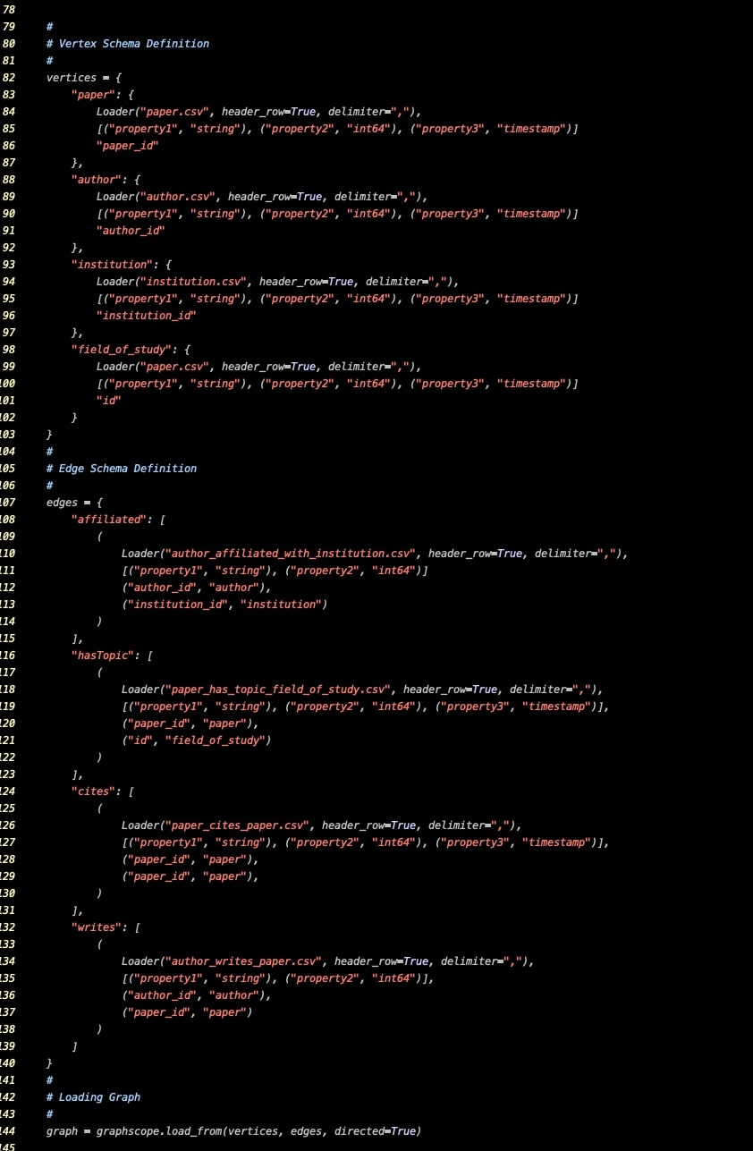
We can see that even for such a flexible language as Python, the schema definition is very complicated for the above-mentioned property graph containing 4 labels, not to mention hundreds of labels of vertices and edges. Even each vertex(edge) may have thousands of properties.
Therefore, in order to reduce the complexity and error rate of the loading process, GraphScope has developed a graphscope-notebook plugin, which can help GraphScope to complete the loading process of complex graph data interactively in the Jupyterlab environment. Currently, the plugin has been deployed in the GraphScope Playground environment, and everyone is welcome to try it out. Next, this article will use this above-mentioned property graph as an example to introduce in detail how to load graph interactively in the Jupyterlab environment.
Plugin Installation
The plugin requires the following conditions:
- JupyterLab >= 3.0
- GraphScope >= 0.12.0
You can install the plugin with the following command:
pip3 install graphscope-notebook
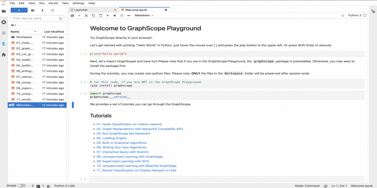
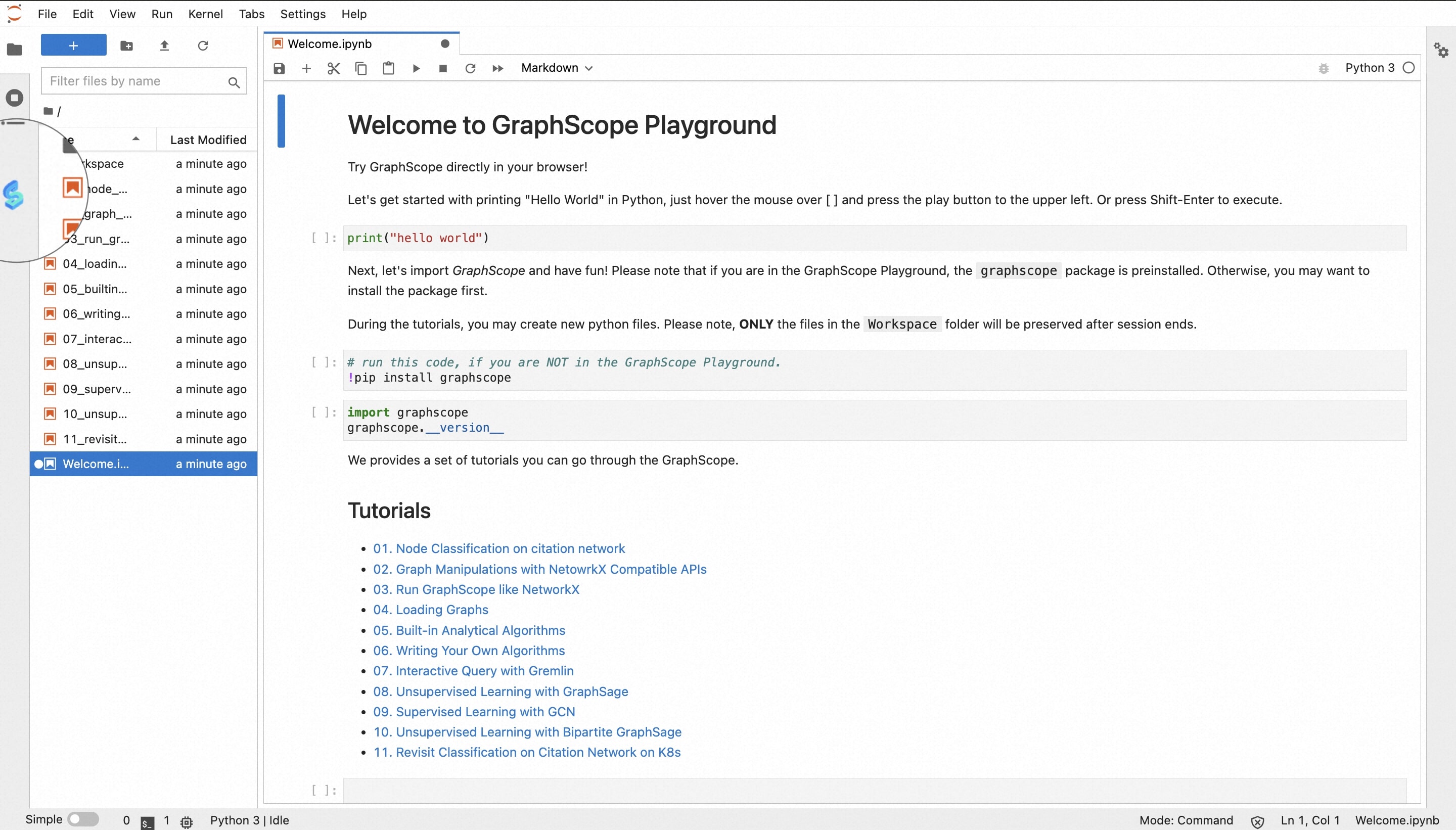
It is worth noting that after the plugin installation is complete, you need to restart Jupyterlab. Finally, if the left sidebar displays as following, it means that the installation is successful; Or you can find it in GraphScope Community to report problems encountered.
Using the Plugin
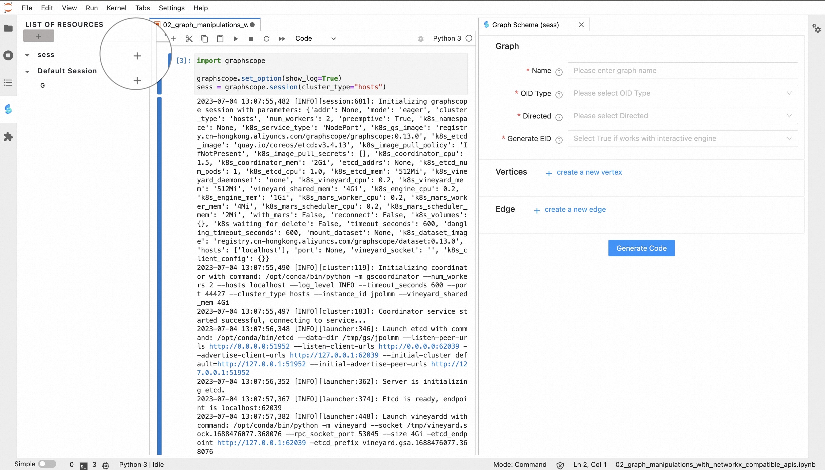
First, we run the following code in the Jupyterlab to create a GraphScope Session.
>>> import graphscope
>> graphscope.set_option(show_log=True)
>>> sess = graphscope.session(cluster_type="hosts")
After the Session is created, we can monitor the resource in the left resource panel. Click the “+” button to open the interactive page on the right side of the notebook:
1. Create Vertex
Next, we can complete the graph data construction according to the prompts on the interactive page. Take the “paper” type of vertex as an example. The page for creating points is as follows. After the information is filled in, click “Create Vertex” to complete the construction of the point.
Next, we can complete the construction of the graph data according to the prompts on the interactive page. Taking the “paper” type of vertex as an example. After filling in the information, click “Create Vertex” to complete the vertex construction.
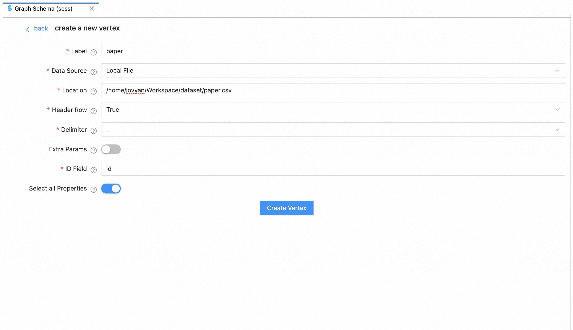
The explanations for each field are as follows:
| field | comment |
|---|---|
| Label | the label of the vertex |
| Data Source | local file represents local data files; online file represents network files, such as OSS, etc. |
| Location | the path of the data source |
| Header Row | If true, the column name will be read from the first row of the source file |
| Delimiter | optional values are “,” “;”, “ “, “\t” |
| Extra Params | additional parameters required by data loading, such as OSS key/secret and endpoint |
| ID Field | which column in the source file is selected as the ID, it can be a number like 0, 1, 2, or a string represents the property name |
| Select all Properties | If true, all properties are loaded, otherwise the properties to be loaded need to be specified |
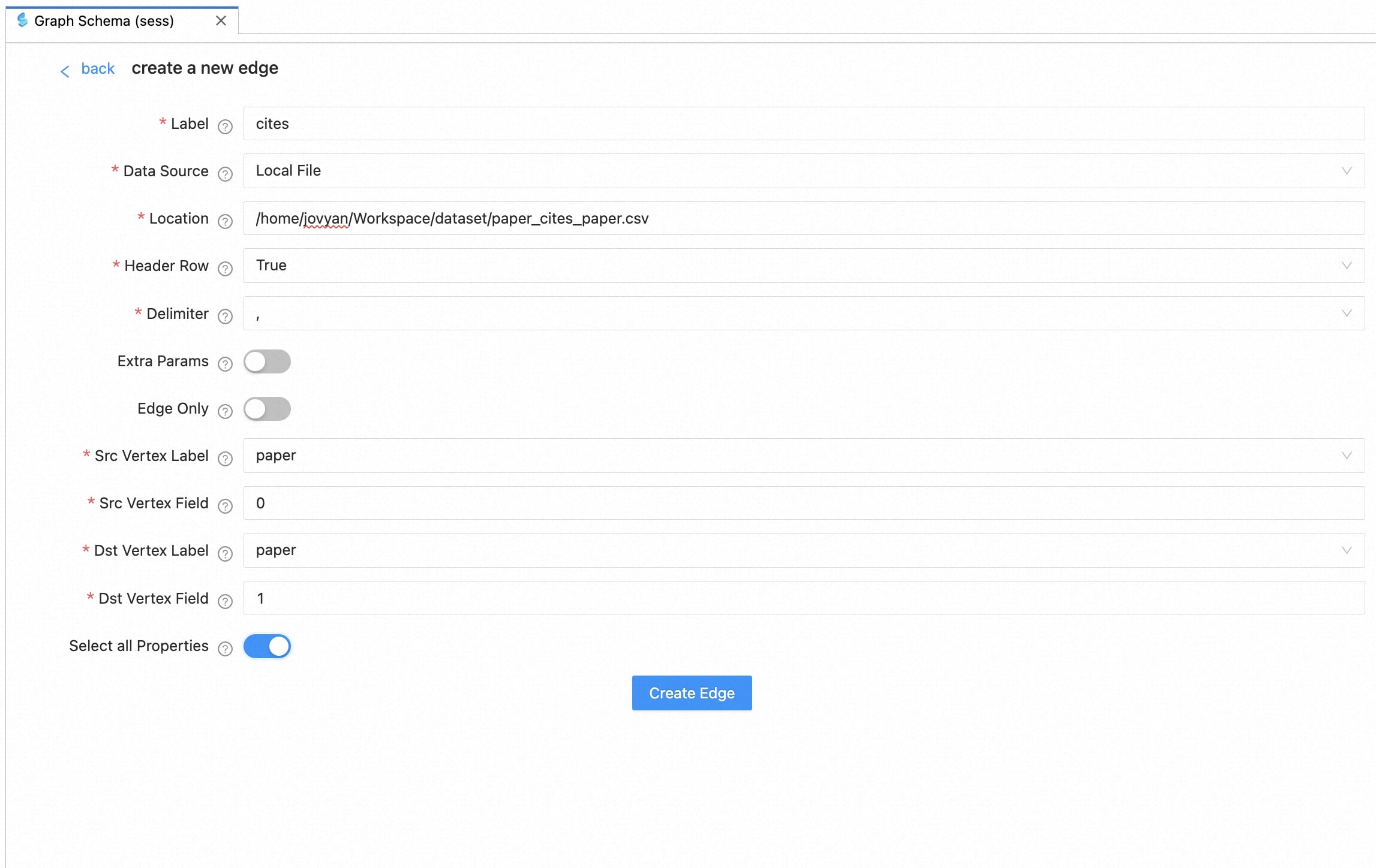
2. Create Edge
Similar to “Create Vertex”, take the “cites” type of edge as an example (paper -> cites -> paper). After the information is filled in, click “Create Edge” to complete the construction of the edge.
| field | comment |
|---|---|
| Edge Only | True for cases where only one edge file and no vertex file |
| Src Vertex Label | the label of source vertex |
| Dst Vertex Label | the label of destination vertex |
| Src Vertex Field | which column used as the ID of the source vertex, it can be a number like 0, 1, 2, or a string represents the property name |
| Dst Vertex Field | which column used as the ID of the destination vertex, it can be a number like 0, 1, 2, or a string represents the property name |
3. Define Graph-Related Information
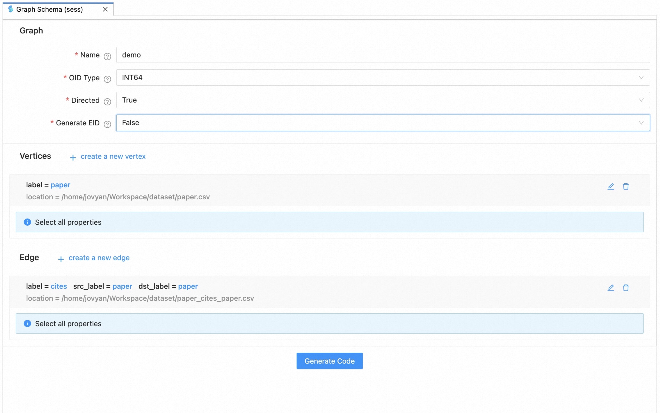
After building all types of vertices/edges, we set the graph-related information:
| field | comment |
|---|---|
| Name | the name of the graph |
| OID Type | the original vertex type of the graph, optional values are “string” and “int64” |
| Directed | whether the graph is directed or not |
| Generate EID | whether to generate a unique id for each edge. Set True if you need to use the GIE service |
4. Generate Code and Load Graph
After all the information above is filled in, select one “Notebook Cell” with the mouse, and click the “Generate Code” button to generate the corresponding graph loading code. Run this cell to finish the data loading process, and monitor the graph resource in the left resource panel:
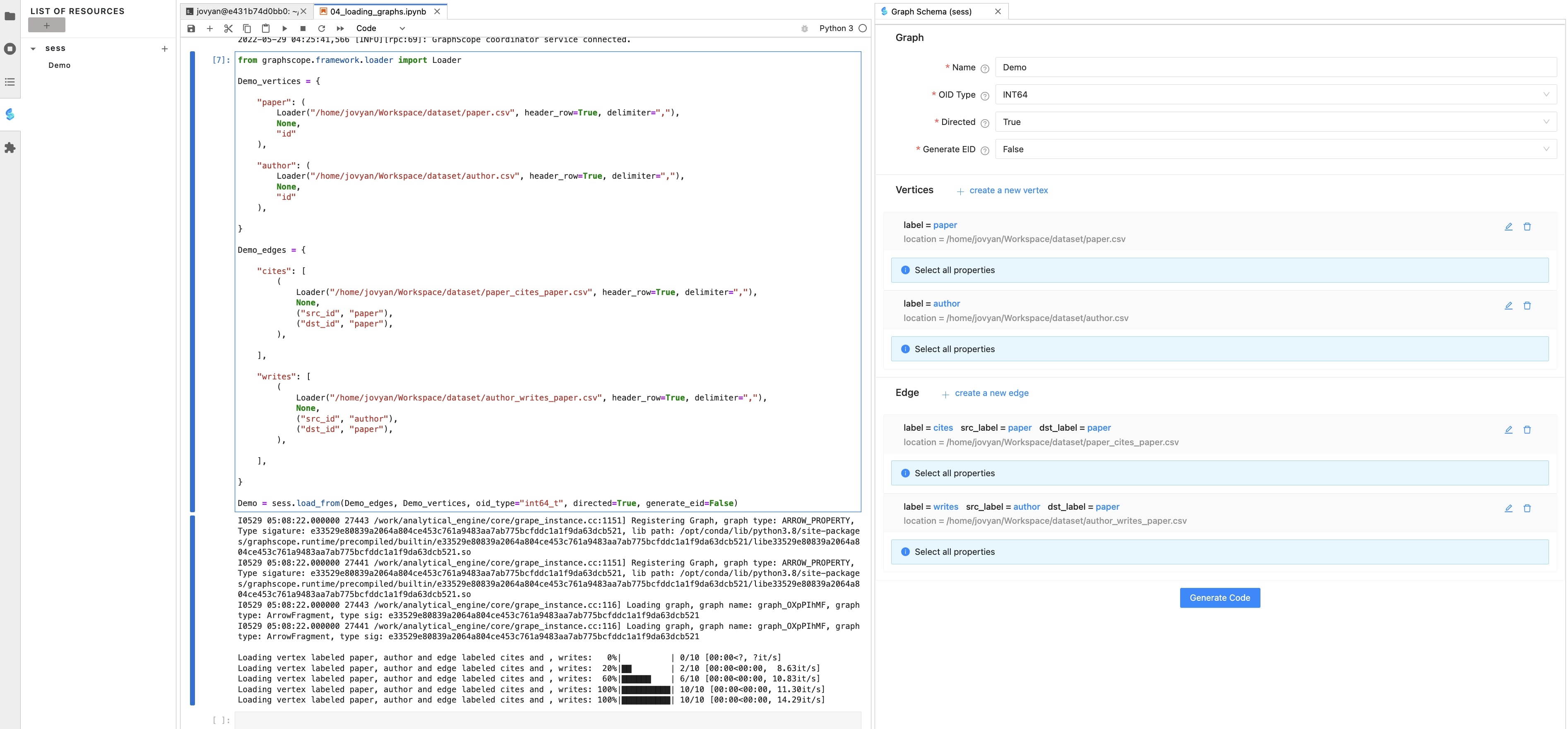
So far, we have successfully used the graphscope-notebook plugin to complete the graph data loading process. Next, we can refer to the documentation to play with GraphScope.
Conclusion
The graphscope-notebook jupterlab plugin currently has the functions of 1) monitoring GraphScope runtime resources; 2) loading graph through an interactive way to reduce the complexity during graph loading process. In addition, we also plan to add visualization analysis of graph data in subsequent versions. Stay tuned!