RelGo: Optimizing Relational Databases with GOpt
 The GraphScope team’s work on proposing RelGo for optimizing SQL/PGQ queries has been accepted by SIGMOD 2025. In this work, RelGo integrates GOpt into relational databases (using DuckDB as an example), enhancing its ability to optimize SQL/PGQ queries and providing better optimization results than DuckDB’s own optimizer.
This article introduces the main content of RelGo.
The GraphScope team’s work on proposing RelGo for optimizing SQL/PGQ queries has been accepted by SIGMOD 2025. In this work, RelGo integrates GOpt into relational databases (using DuckDB as an example), enhancing its ability to optimize SQL/PGQ queries and providing better optimization results than DuckDB’s own optimizer.
This article introduces the main content of RelGo.
1. Background and Motivations
In the realms of data management and analytics, relational databases have long been the bedrock of structured data storage and retrieval, empowering a plethora of applications, across domains ranging from finance to healthcare. To facilitate tasks like creating tables and retrieving information in a database, the Structured Query Language (SQL) was developed and has been widely adopted by various Relational Database Management Systems (RDBMS). Below is an example of querying on IMDB data with an SQL query:
Query 1 (Q1)

SELECT n.name
FROM NAME AS n1,
     CAST_INFO AS ci1,
     CAST_INFO AS ci2,
     TITLE AS t1,
     TITLE AS t2,
     MOVIE_COMPANIES AS mc1,
     MOVIE_COMPANIES AS mc2,
     COMPANY_NAME AS cn
WHERE n1.id = ci1.person_id
      AND ci1.movie_id = t1.id
      AND t1.id = mc1.movie_id
      AND mc1.company_id = cn.id
      AND n1.id = ci2.person_id
      AND ci2.movie_id = t2.id
      AND t2.id = mc2.movie_id
      AND mc2.company_id = cn.id
      AND t1.title <> t2.title;
The relationships between the tables relevant to Q1 in IMDB are illustrated in the following ER diagram
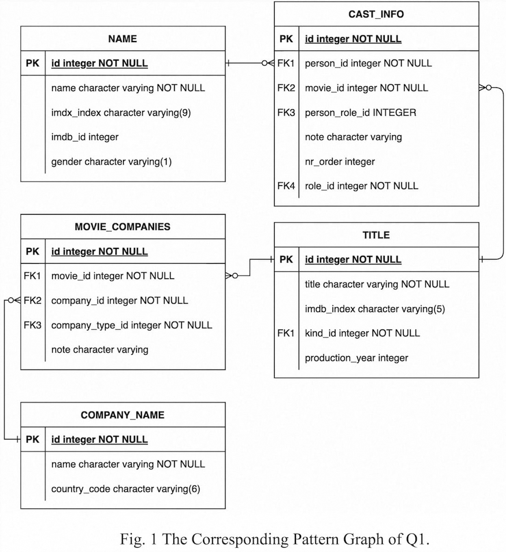
The NAME table and TITLE table store information about persons and movies, respectively. The CAST_INFO table holds the quaternary relationship between persons, movies, roles (characters played in the movies), and professions (such as actor, actress, director, writer, etc.). The COMPANY_NAME table contains the names of movie companies, while the MOVIE_COMPANIES table records the association between movies, movie companies, and company types. Therefore, the SQL query above aims to find individuals who have participated in the production of at least two movies for the same company.
It’s easy to see that using SQL to describe such queries can sometimes result in very lengthy statements, especially when there’s a need to describe the relationships between tables.
Another more intuitive example is finding n persons who all know each other. Each time we describe the mutual relationship between two persons, we need to add two join conditions. For example:
Person1.id = Knows.person1id AND Person2.id = Knows.person2id
Hence, describing n persons knowing each other requires writing at least $n \times (n-1)$ join conditions. Manually writing such query statements is evidently very inefficient.
When a query requires describing the relationships between tables, using graph queries can be relatively more convenient. The advantage lies in being able to express the query in a graph-like manner. Using Cypher as an example, query Q1 can be expressed as follows:
MATCH (n1:NAME)-[ci1:CAST_INFO]->(t1:TITLE)-[mc1:MOVIE_COMPANIES]->(cn:COMPANY_NAME),
      (n1)-[ci2:CAST_INFO]->(t2:TITLE)-[mc2:MOVIE_COMPANIES]->(cn)
WHERE t1.title <> t2.title
RETURN n1.name;
This query intuitively describes the following graph pattern:
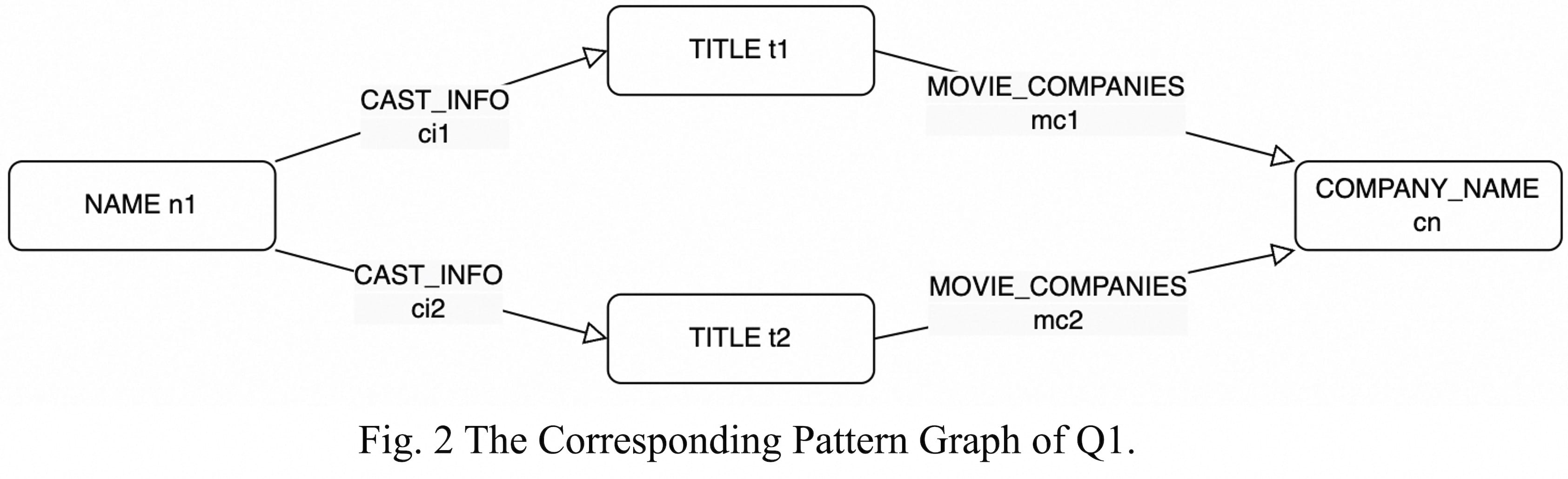
For the scenario of finding n persons knowing each other, using a graph query only requires describing a complete graph with n vertices (i.e., an n-clique). The above example demonstrates that using graph queries can significantly reduce the time database users spend writing SQL, allowing them to express their intended queries more quickly and conveniently.
Therefore, in ISO SQL:2023, an extension called SQL/PGQ (SQL/Property Graph Queries) has been introduced to support graph queries within SQL expressions. Assuming that each tuple in the NAME, TITLE, and COMPANY_NAME tables represents a vertex, and each tuple in the CAST_INFO and MOVIE_COMPANIES tables represents an edge, we can rewrite query Q1 as follows in SQL/PGQ:
SELECT n_name FROM GRAPH_TABLE (G
    MATCH (n1:NAME)-[ci1:CAST_INFO]->(t1:TITLE)-[mc1:MOVIE_COMPANIES]->(cn:COMPANY_NAME),
      (n1)-[ci2:CAST_INFO]->(t2:TITLE)-[mc2:MOVIE_COMPANIES]->(cn)
    WHERE t1.title <> t2.title
    COLUMNS (n1.name AS n_name)
) g;
The SQL/PGQ extension addresses how to write graph queries within SQL expressions. However, once we get the SQL/PGQ query statements, analyzing and optimizing them remains a new challenge brought by SQL/PGQ. Query optimization refers to finding an efficient query plan based on a user-given query to achieve better query performance. Research on relational database query optimizers is typically carried out for the SPJ (selection-projection-join) queries. However, SQL/PGQ queries cannot be expressed as SPJ queries, because the GRAPH_TABLE clause cannot be directly represented through traditional selection, projection, and join operators. Therefore, it is challenging to directly use traditional relational database optimizers to optimize SQL/PGQ statements.
Addressing this issue, we introduce a new query skeleton called SPJM (selection-projection-join-matching) and subsequently designed and implemented a converged optimization framework named RelGo based on GOpt. Our main contributions can be summarized as follows:
- We define RGMapping to map relational tables to a property graph based on SQL/PGQ statements. Using RGMapping, we have defined a new query skeleton called SPJM, which can be used to express queries that contain both relational and graph queries.
- We have developed a theory to transform SPJM queries into SPJ queries, allowing existing relational databases to directly handle SPJM queries. This approach is called the graph-agnostic approach. We have demonstrated that this graph-agnostic method has a significantly larger search space (exponentially larger) compared to our method in some scenarios.
- We have designed and implemented RelGo to leverage relational and graph query optimization techniques to optimize SPJM queries. In detail, RelGo employs state-of-the-art graph optimization techniques and implements graph-related physical operations based on graph indexes.
- We developed RelGo by integrating it with the industrial relational optimization framework Calcite, and employing DuckDB for execution runtime. We conducted extensive experiments to evaluate its performance. The results on the LDBC Social Network Benchmark indicate that RelGo significantly surpasses the performance of the graph-agnostic baseline, achieving an average speedup of 21.9x over the baseline, which remains 5.4x faster even when graph indexing is enabled.
This work has been accepted at SIGMOD 2025 (https://dl.acm.org/doi/10.1145/3698828,https://arxiv.org/pdf/2408.13480).
2. Concepts and SPJM Skeleton
Let’s start by briefly explaining some of the concepts that will be used in this blog, including Property Graph and RGMapping. In this blog, for the sake of convenience, we will use the terms “table” and “relation” interchangeably.
2.1 Concepts
Given an expression that contains both relational queries and graph queries, in order to integrate the query plans of both, it’s necessary to define a method for translating between relational data and graph data. Therefore, we use the following concepts.
Property Graph
A property graph is composed of vertices and edges, where vertices and edges can have various attributes. In the upper right corner of Figure 3(a), an example of a property graph is provided. This property graph contains a total of 5 vertices, including 3 Persons and 2 Messages. Additionally, the property graph includes 8 edges, each tagged with either Knows or Likes.
RGMapping
RGMapping maps tuples from relational tables to vertices or edges in a property graph. Specifically, RGMapping includes a vertex mapping and an edge mapping, which respectively map tuples from tables to different vertices and edges. To more conveniently describe the definition of RGMapping, we will illustrate this with the following figure.
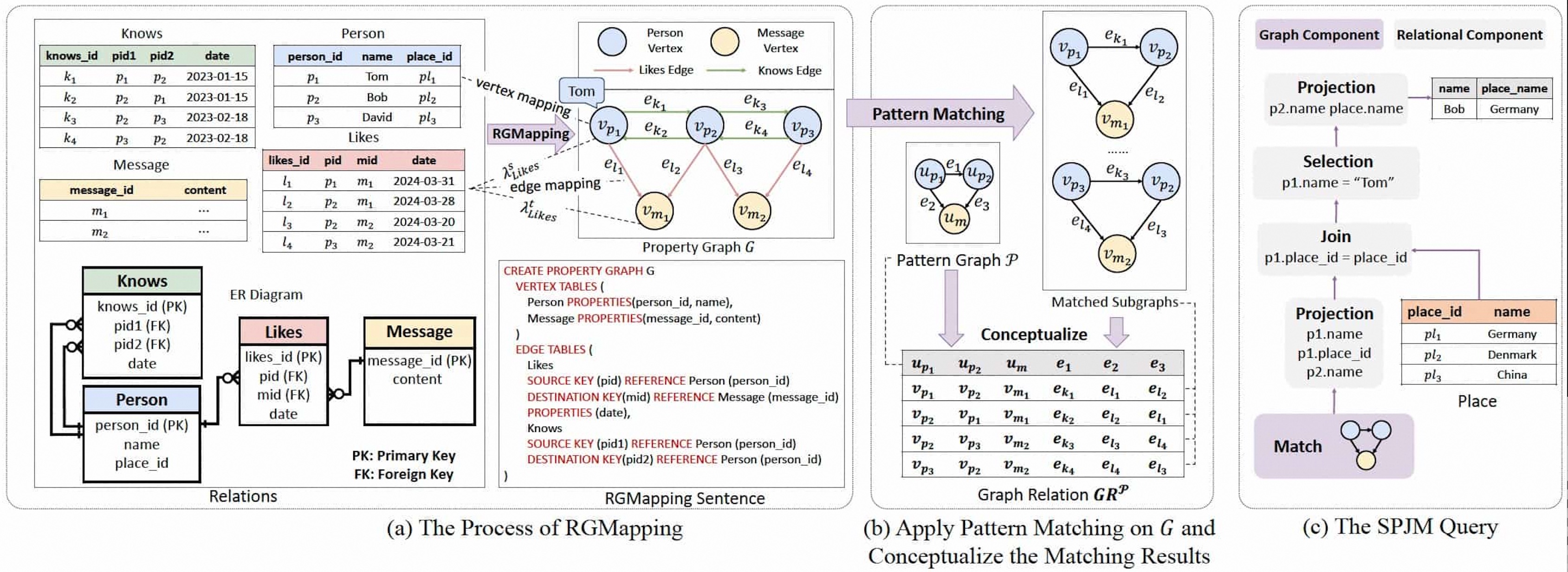

Fig. 3(a) contains four relational tables: Knows, Person, Likes, and Message. The relationships between them can be described using the ER diagram in the bottom left corner of Fig. 3(a). In relational data modeling, an ER diagram includes entities and relationships. Consequently, vertices can be mapped from relations corresponding to entities, and edges can be mapped from relations corresponding to relationships. In this example, tuples in the Person and Message tables are mapped to vertices, while tuples in the Knows and Likes tables are mapped to edges. The resulting property graph is shown in the upper right corner of Figure 3(a), labeled as property graph G.
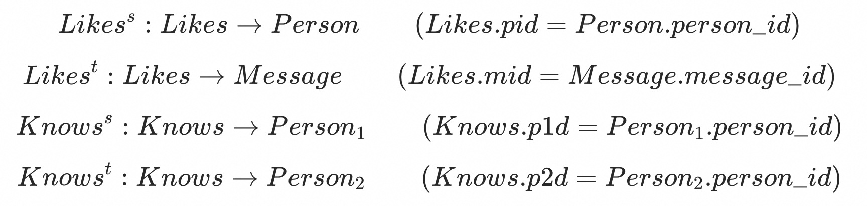
In the property graph G, p1 represents the tuple with person_id = 1 in the Person table, and k1 represents the tuple with knows_id = 1 in the Knows table. RGMapping is used to define the mapping relationships between relational tables and the property graph. For ease of explanation, we will refer to tables mapped to vertices as vertex tables and tables mapped to edges as edge tables. For edge tables, it is not sufficient to just know the mapping relationship between a tuple and an edge; it is also necessary to know the association between the edge’s source and target vertices and the vertex tables. Specifically, for the edge table Likes in this example, we can provide the following two association relationships:
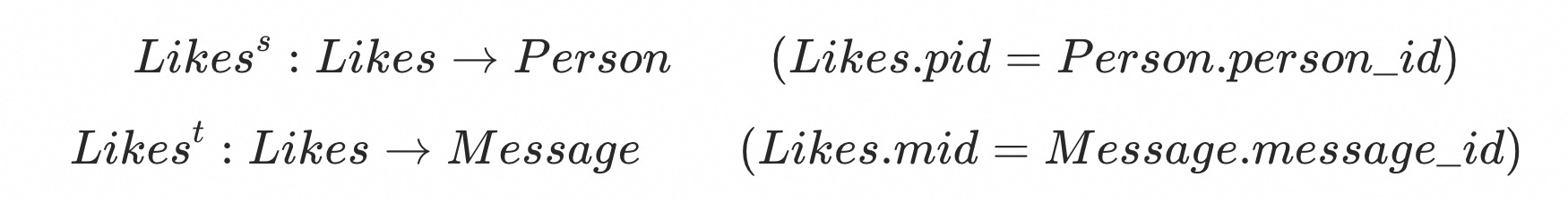
These two association relationships respectively indicate that for a tuple in the Likes table, which corresponds to an edge in the property graph, the source vertex of the edge corresponds to a tuple in the Person table, and the target vertex corresponds to a tuple in the Message table. The correspondence between tuples is determined based on the values of Likes.pid, Person.person_id, and Message.message_id. Specifically, a tuple in the Likes table is associated with a tuple in the Person table if and only if the value of the pid attribute matches the value of the person_id attribute. For example, the first row in the Likes table is associated with the first row in the Person table, because l1.pid = p1.person_id. It means that the source vertex of the edge mapped from the first row of Likes is mapped from the first row of Person.
Generally, this association can be derived from the primary-foreign key relationships between relational tables. Specifically, because the Likes table has foreign keys pid and mid pointing to the Person and Message tables, respectively, the vertex tables related to Likes are Person and Message.
With this information, it is possible to convert between relational tables and vertices and edges in the property graph. Therefore, given a relational database, as long as the corresponding RGMapping is defined, part of the relational tables can be converted into a property graph, thereby leveraging the capabilities of a graph optimizer in query optimization.
2.2 SPJM Skeleton
To represent graph queries, we introduce a new operator into the relational operators, namely the Matching Operator. This operator takes a graph relation and a pattern graph as input and produces a graph table as output. Here, a graph relation is a special type of table. Each tuple in this relation represents a property graph, with each attribute value of the tuple corresponding to a vertex or edge. The table shown at the bottom of Fig. 3(b) is an example of a graph relation.
For each tuple (i.e., property graph) in the input graph relation, the Matching Operator searches for all subgraphs isomorphic to the input pattern graph. Each row of the graph relation returned by the Matching Operator corresponds to one such found isomorphic subgraph. In this paper, we consider queries that include selection, projection, join, and matching operators. Queries composed of these operators are referred to as SPJM queries.
3. Optimizing Matching Operator
In this section, we focus on handling the matching operator, which plays a distinct role within the SPJM queries. We discuss two main perspectives of optimizing the matching operator: logical transformation and physical implementation. Logical transformation is responsible for transforming a matching operator into a logically equivalent representation, while physical implementation focuses on how the matching operator can be efficiently executed.
3.1 Logical Transformation
Given a matching operator, suppose the input pattern graph is as follows:
MATCH (p1:PERSON)-[e1:KNOWS]->(p2:PERSON)-[e3:LIKES]->(m:MESSAGE),
      (p1)-[e2:LIKES]->(m)
RETURN p1.name, p1.place_id, p2.name
This pattern graph, as shown in Figure 3(b), searches for two persons who like the same message. The table names in the pattern graph use uppercase letters, such as PERSON. For this query, we propose two transformation methods: one is the graph-agnostic approach, and the other is the graph-aware approach.
3.1.1 Graph-Agnostic Approach
The graph-agnostic approach directly converts the pattern graph into joins between tables based on the RGMapping, thus transforming the SPJM problem into an SPJ problem. Existing relational optimizers can then be used for query optimization. According to the RGMapping described in Section 2 and the ER diagram in Figure 3(a) that describes the relationships between the tables, it is easy to determine that the Person, Message, Knows, and Likes tables are respectively mapped to vertices or edges labeled Person, Message, Knows, and Likes in the graph.
Moreover, the following association relationships exist between the vertex tables and edge tables:
Here, $Person_1$ and $Person_2$ represent two copies of the Person table, containing the same content as the original Person table. Subsequently, each edge in the pattern graph can be obtained through joins between the vertex tables and edge tables. Specifically, the edges in the aforementioned pattern graph can be converted into the following joins:
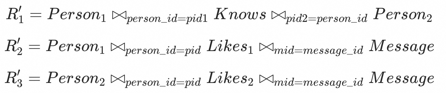
Therefore, the matching operator can be converted to:
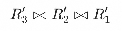
Then, relational optimizers can be used to optimize the query.
3.1.2 Graph-Aware Approach
In this section, we introduce a graph-aware transformation that incorporates key ideas from the literature on graph optimization. Specifically, we first decompose the pattern graph in Figure 3(b) to obtain the following decomposition tree.
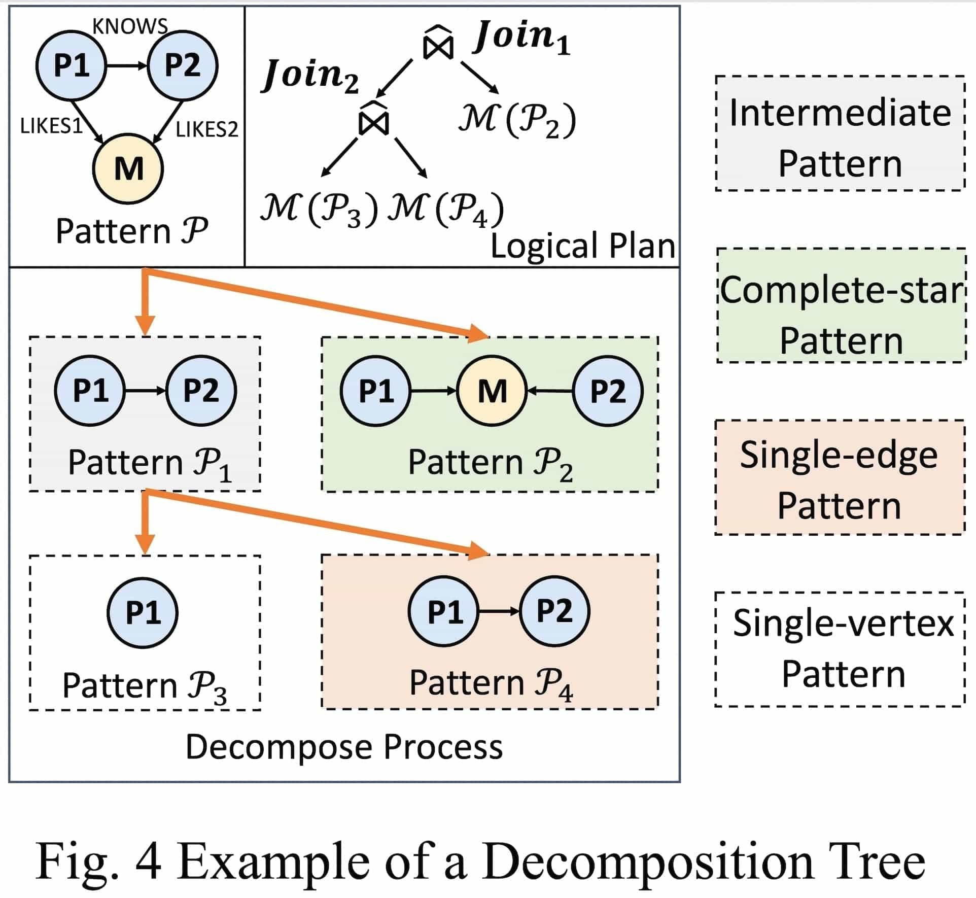
In detail, the tree has a root node that represents the pattern graph, and each non-leaf intermediate node is a sub-pattern (a subgraph of the pattern) , which has left and right child nodes. These two child nodes are both subgraphs of the intermediate node, and by joining the two child nodes, we obtain this intermediate node. Following state-of-the-art graph optimizers, to guarantee a worst-case optimal execution plan, all intermediate sub-patterns in the decomposition tree must be induced subgraphs of the pattern graph.
The leaf nodes of the decomposition tree must be Minimum Matching Components (MMCs). An MMC can either be a single-vertex pattern or a complete-star pattern. A complete-star pattern must be located in the right subtree, with all the leaf nodes of the star appearing in the left subtree. It is easy to see that a single-edge pattern is a special type of complete-star pattern. This design is mainly to ensure that the execution plan is worst-case optimal.
The decomposition tree in Fig. 4 contains three MMCs: $\mathcal{P}_2$ (complete-star pattern), $\mathcal{P}_3$ (single-vertex pattern subgraph), and $\mathcal{P}_4$ (single-edge pattern subgraph). After decomposing, for each node in the decomposition tree, we join its left and right child nodes to obtain the result of the current node. For example, when matching the property graph G in Fig. 3(a) with the pattern graph in Fig. 4, the matching result of $\mathcal{P}_1$ is (p1, k1, p2), (p2, k2, p1), (p2, k3, p3), (p3, k4, p2). The matching result of $\mathcal{P}_2$ is (p1, l1, m1, l2, p2), (p2, l2, m1, l1, p1), (p2, l3, m2, l4, p3), (p3, l4, m2, l3, p2).
By joining these results on vertices $\mathcal{P}_1$ and $\mathcal{P}_2$ in the pattern, we obtain (p1, k1, p2, l1, m1, l2), (p2, k2, p1, l2, m1, l1), (p2, k3, p3, l3, m2, l4), and (p3, k4, p2, l4, m2, l3). These results are exactly the results of matching the original pattern graph $\mathcal{P}$, as shown in the table below Fig. 3(b).
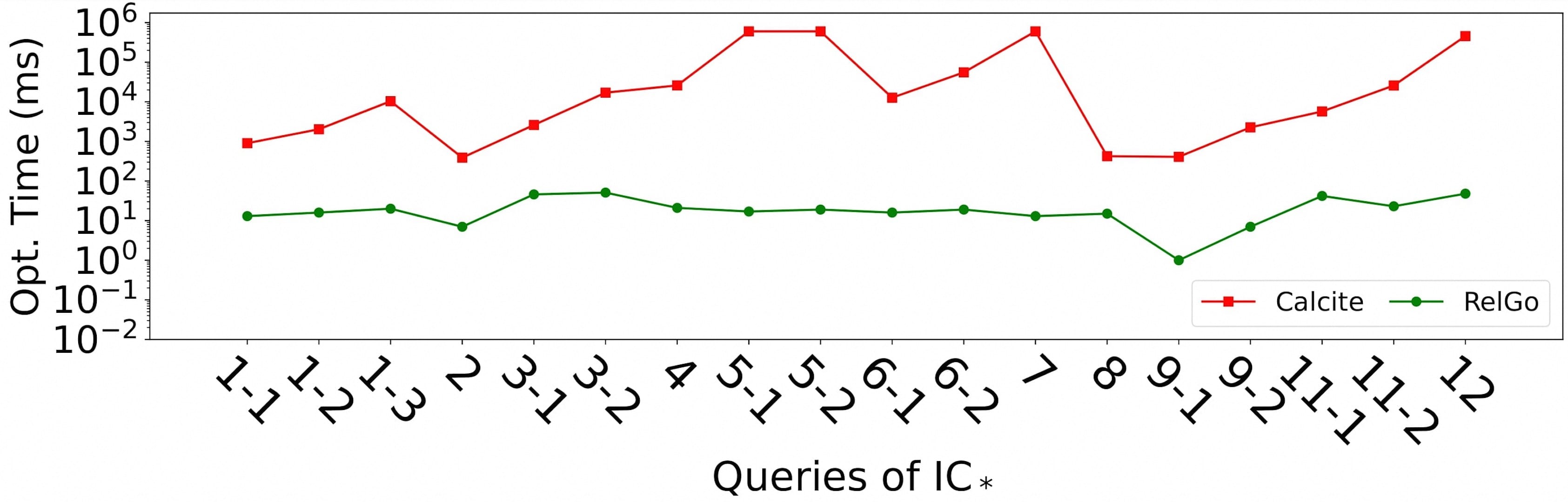
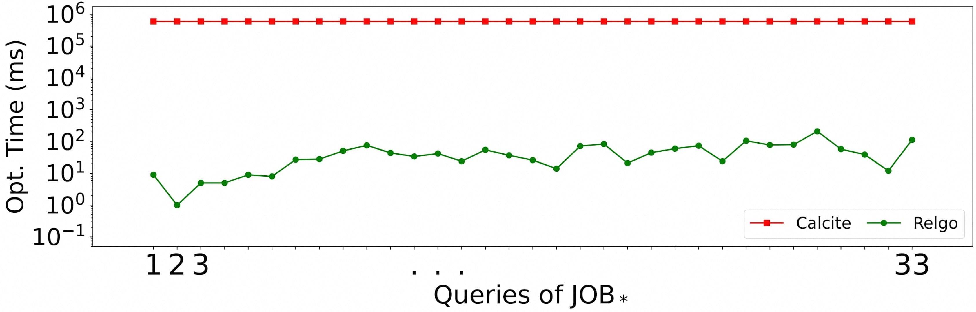
We have demonstrated that in some scenarios, the search space of the graph-aware approach is exponentially smaller than that of the graph-agnostic approach. Taking RelGo (graph-aware approach) and Calcite (graph-agnostic approach) as examples, we conducted experiments on the LDBC SNB benchmark (on LDBC30 dataset) and JOB benchmark (on IMDB dataset) to compare their optimization times. The experimental results show that RelGo significantly improves optimization speed compared to Calcite.

3.2 Physical Implementation
Physical implementation optimization refers to using efficient physical implementations when realizing the operators in the execution plan to make the actual execution more efficient. Referencing GRainDB, we implemented a graph index. The following illustration is an example of a graph index.
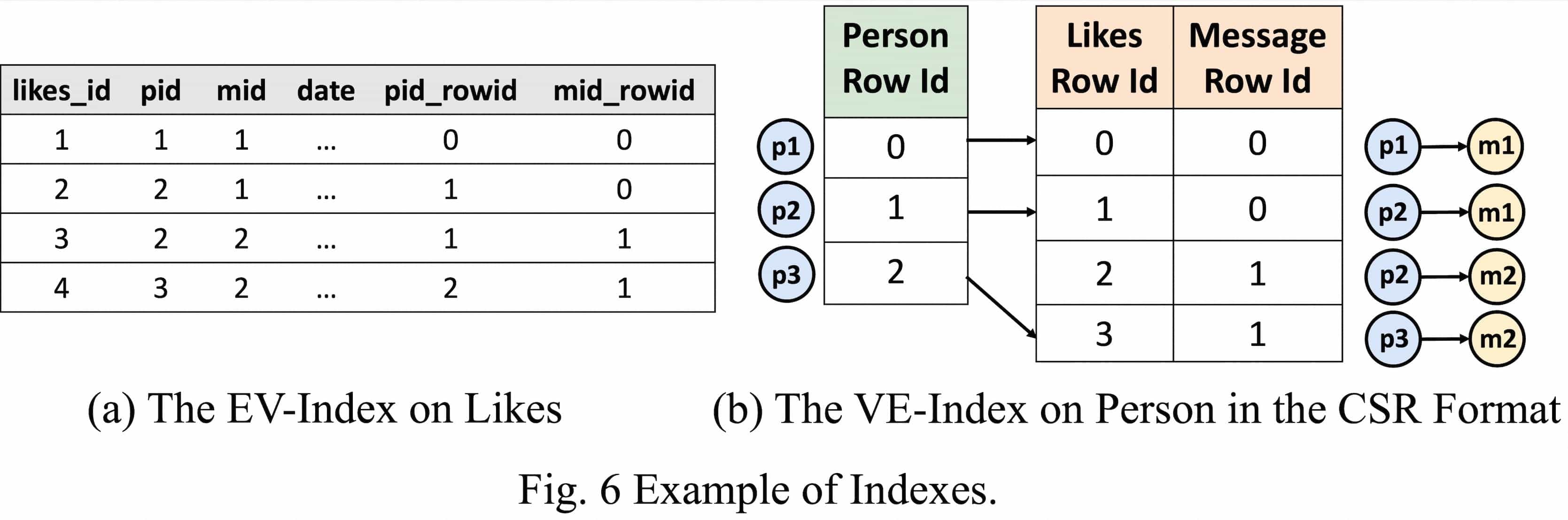
As shown in Fig. 6, the EV index is built on the edge table. For each tuple in the Likes table (which is an edge table), two new attribute columns, pid_rowid and mid_rowid, are added to record the positions (i.e., row numbers) of the source and target vertices of the corresponding edge in the respective vertex tables. For example, l1 in the Likes table corresponds to an edge whose source vertex is located at the 0-th row of the Person table and whose target vertex is at the 0-th row of the Message table.
The VE index is built based on the vertex tables. For each tuple in the Person table, the VE index records the positions of its adjacent edges in the edge table (i.e., row numbers) and the positions of the other endpoints of these edges in the corresponding vertex tables. Specifically, for tuple p1 in the Person table, the VE index records its adjacent edge’s position at the 0-th row of the Likes table and the other endpoint of that edge at the 0-th row of the Message table.
Based on these two indexes, when actually joining the vertex and edge tables, it is possible to skip value comparisons and quickly obtain tuples that can be joined.
Specifically, we implemented three main types of physical implementation optimizations for the decomposition tree:
- Given an intermediate node, when its right subtree is an MMC containing only a single edge, the join of its left and right subtrees can be implemented as a combination of the EXPAND_EDGE and GET_VERTEX operators, without flattening the result during the computation of these two operators. For example, consider Figure 5. Suppose a decomposition tree has an intermediate node
(:PERSON) JOIN (:PERSON)-[:LIKES]->(:MESSAGE). In this case, both the left and right subtrees are MMCs, i.e.,(:PERSON)and(:PERSON)-[:LIKES]->(:MESSAGE). Assume that a tuple from the matching results of the left subtree is (p2). When joined with the right subtree, the result is (p2, [l2, l3], [m1, m2]). After flattening, the resulting tuples are (p2, l2, m1) and (p2, l3, m2). - Given an intermediate node, when its right subtree is a complete-star pattern, we implemented the EXPAND_INTERSECT operator to avoid flattening the results during computation. Consider the intermediate node
(:PERSON)-[:KNOWS]->(:PERSON) JOIN (:PERSON)-[:LIKES]->(:MESSAGE)<-[:LIKES]-(:PERSON), which corresponds to the two child nodes of the root in the decomposition tree shown in Fig. 4. Suppose a tuple from the matching results of the left subtree is (p1, k1, p2), then the EXPAND_INTERSECT operator first applies the EXPAND_EDGE and GET_VERTEX operators on p1 and p2, yielding the results (p1, k1, p2, [l1], [m1]) and (p1, k1, p2, [l2, l3], [m1, m2]). Subsequently, it directly intersects these results to obtain (p1, k1, p2, [(l1, l2, m1)]). Finally, flattening this yields the result (p1, k1, p2, l1, l2, m1). - Whenever possible, use graph indices in the physical implementation to accelerate joins between vertex tables and edge tables.
4. The Converged Optimization Framework: RelGo
In this section, we specifically introduce the proposed converged optimization framework, RelGo, with its optimization workflow as follows:
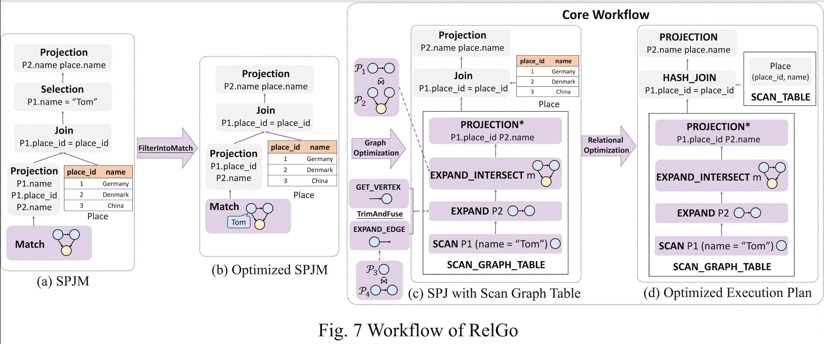
As illustrated in Fig. 7, the core workflow of the RelGo framework consists of two components: graph optimization and relational optimization. The graph optimization is responsible for handling the graph component in an SPJM query, leveraging graph optimization techniques to determine the optimal decomposition tree of the matching operator. On the other hand, the relational optimization takes over to optimize the relational component in the query. The order in which these two components are applied is not strictly defined. However, for the purpose of our discussion, we will first focus on the graph optimization and then proceed to the relational optimization.
RelGo uses GOpt for graph optimization and applies techniques such as FilterIntoMatchRule TrimAndFuseRule during the optimization process. Specifically, the TrimAndFuseRule describes a scenario where the EXPAND_EDGE and GET_VERTEX operators, when executed consecutively without the need to retrieve edge properties, become equivalent to a direct neighbor retrieval operator. Therefore, if the corresponding graph index is constructed, the VE index can be utilized to merge the two operators into a single EXPAND operator, directly retrieving the neighboring vertices.
Once the graph optimizer has computed the optimal execution plan for the matching operator, the next step is to integrate this plan with the remaining relational operators in the SPJM query. The relational optimization is responsible for optimizing these remaining operators, which are all relational operators.
Specifically, to prevent the relational optimizer from delving into the internal details of the graph pattern matching process, we introduce a new physical operator called SCAN_GRAPH_TABLE, as shown in Fig. 7(c), which encapsulates the optimal execution plan for the matching operator.
The SCAN_GRAPH_TABLE operator acts as a bridge between the graph and relational components of the query. From the perspective of the relational optimizer, SCAN_GRAPH_TABLE behaves like a standard SCAN operator, providing a relational interface to the matched results.
We engineered the frontend of RelGo in Java and built it upon Apache Calcite to utilize its robust relational query optimization infrastructure. Firstly, we enhanced Calcite’s SQL parser to recognize SQL/PGQ extensions, specifically to parse the GRAPH_TABLE clause. We created a new ScanGraphTableRelNode that inherits from Calcite’s core RelNode class, translating the GRAPH_TABLE clause into this newly defined operator within the logical plan. Secondly, we incorporate heuristic rules such as FilterIntoMatchRule and TrimAndFuseRule into Calcite’s rule-based HepPlanner, by specifying the activation conditions and consequent transformations of each rule. For more nuanced optimization, we rely on the VolcanoPlanner, the cost-based planner in Calcite, to optimize the ScanGraphTableRelNode. We devised a top-down search algorithm that assesses the most efficient physical plan based on a cost model, combined with high-order statistics from GLogue for more accurate cost estimation. Lastly, the converged optimizer outputs an optimized and platform-independent plan formatted with Google Protocol Buffers (protobuf), ensuring the adaptability of \name’s output to various backend database systems
We developed the RelGo framework’s backend in C++ using DuckDB as the relational execution engine to showcase its optimization capabilities. We integrated graph index support in GRainDB. Besides, we craft a new join on DuckDB called EI-Join for the support of EXPAND_INTERSECT. Without graph index, the HASH_JOIN operator is used throughout the entire plan.
5. Experiments
To evaluate the quality of the query plans generated by RelGo, we conducted performance testing using two datasets: LDBC and IMDB. The experiments were carried out on the LDBC SNB and JOB benchmarks. The LDBC dataset was generated by the official LDBC Data Generator with scale factors of 10, 30, and 100. The JOB benchmark queries were executed on the IMDB dataset. The baseline methods compared in the experiments include:
- DuckDB:Common relational databases that use graph-agnostic methods for optimization.
- GRainDB:GRainDB implements graph indexes on DuckDB. After optimizing the queries using DuckDB’s optimizer, some join operators are replaced with predefined joins utilizing the graph indexes.
- Umbra:Its query optimizer can generate query plans that include worst-case optimal joins.
- Kùzu: Graph database management systems using the property graph model.
The experimental results are as follows:
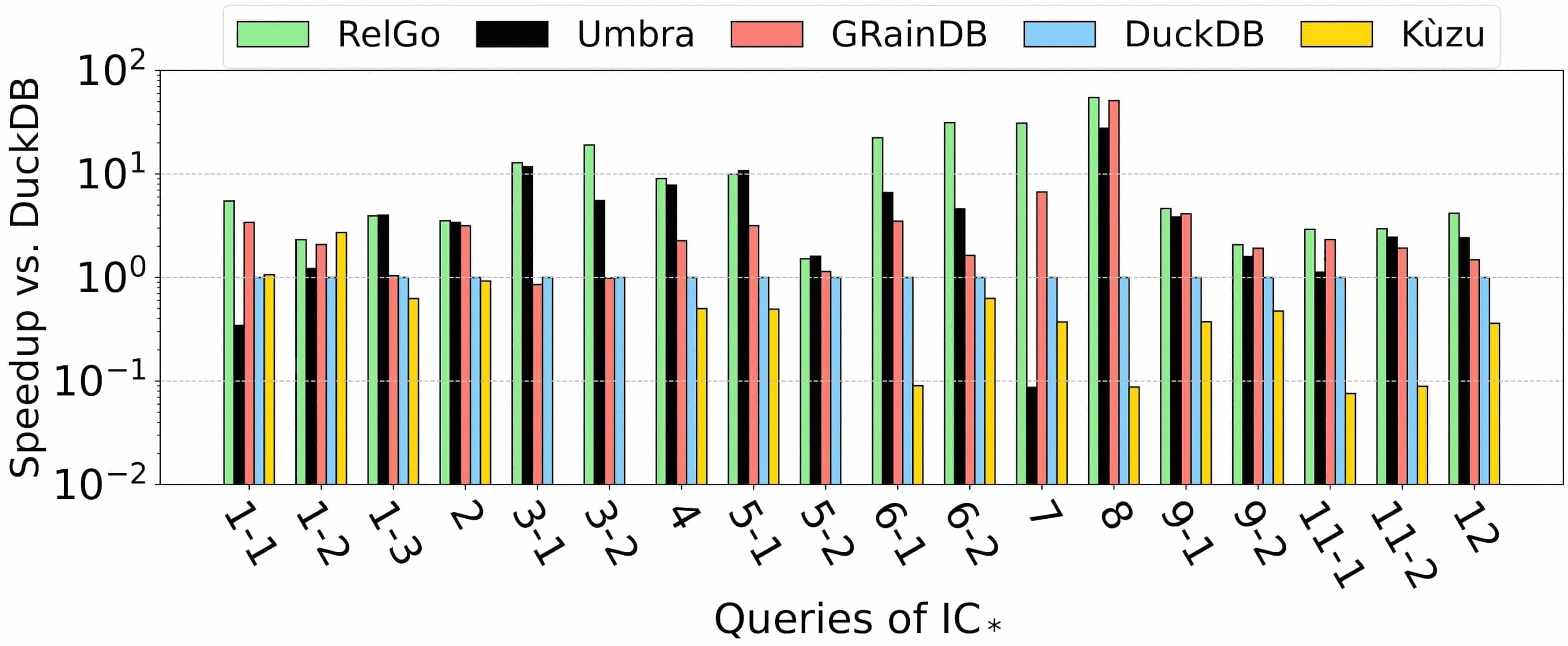 LDBC10
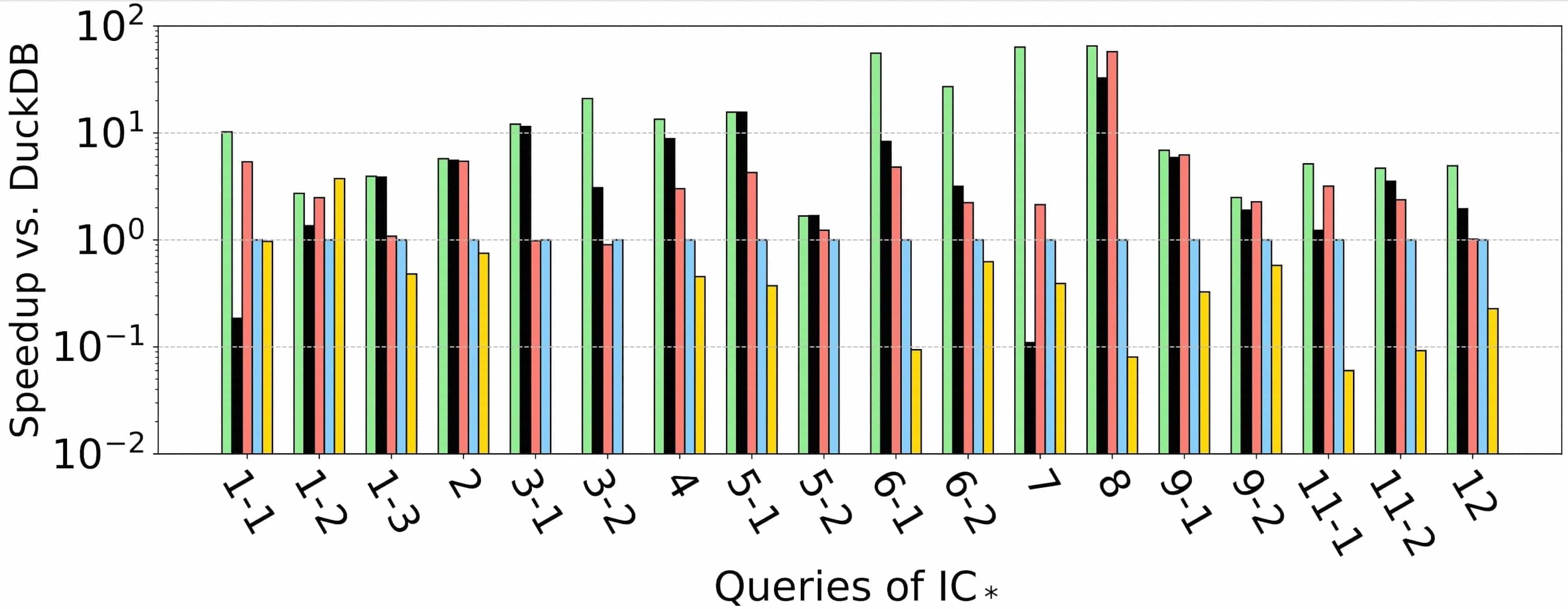 LDBC30
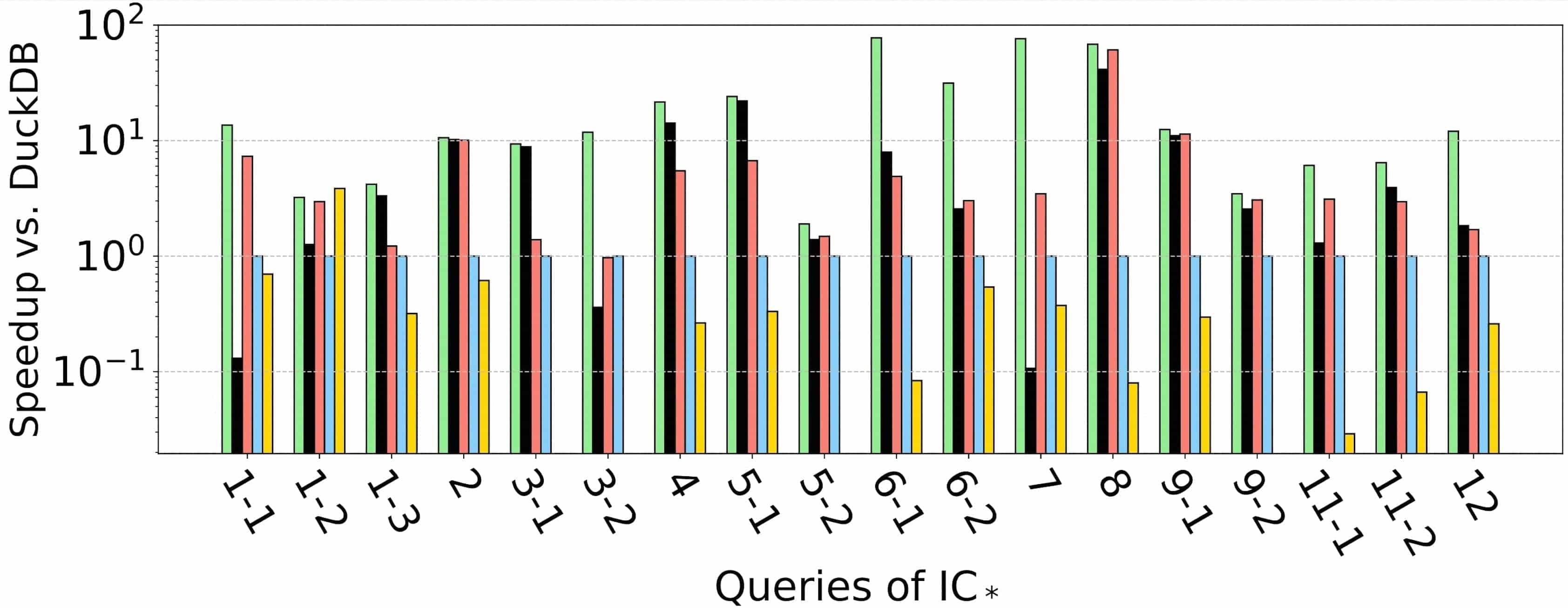 LDBC100
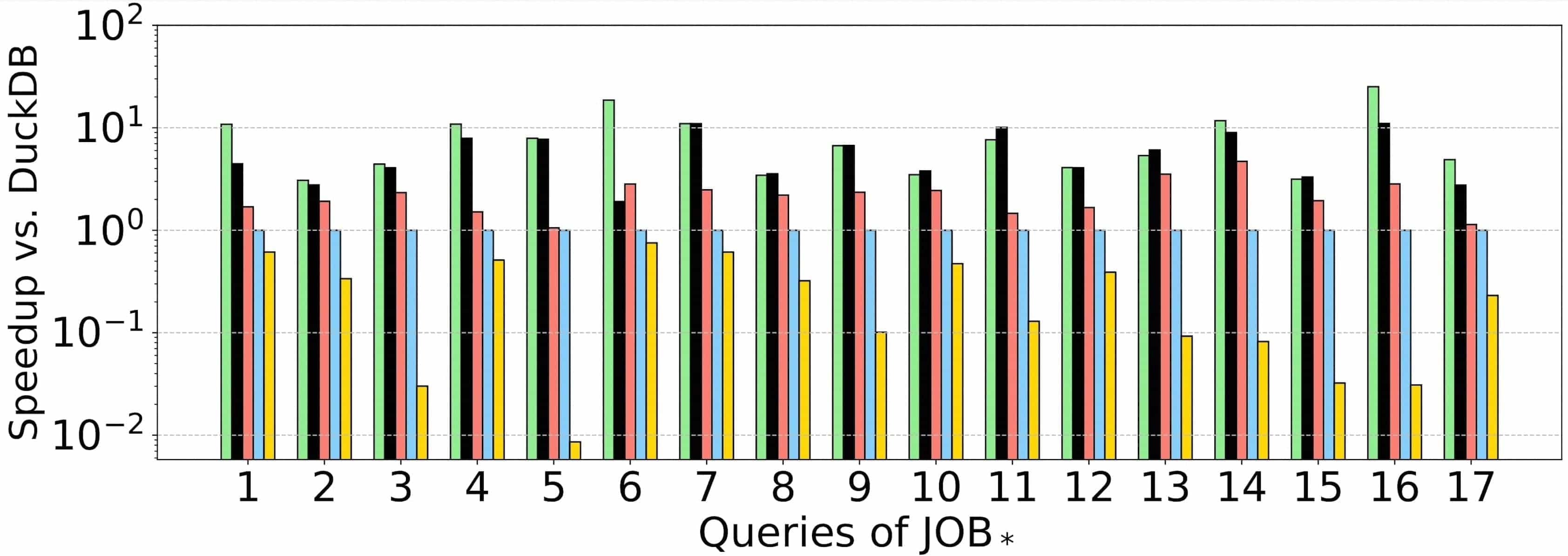
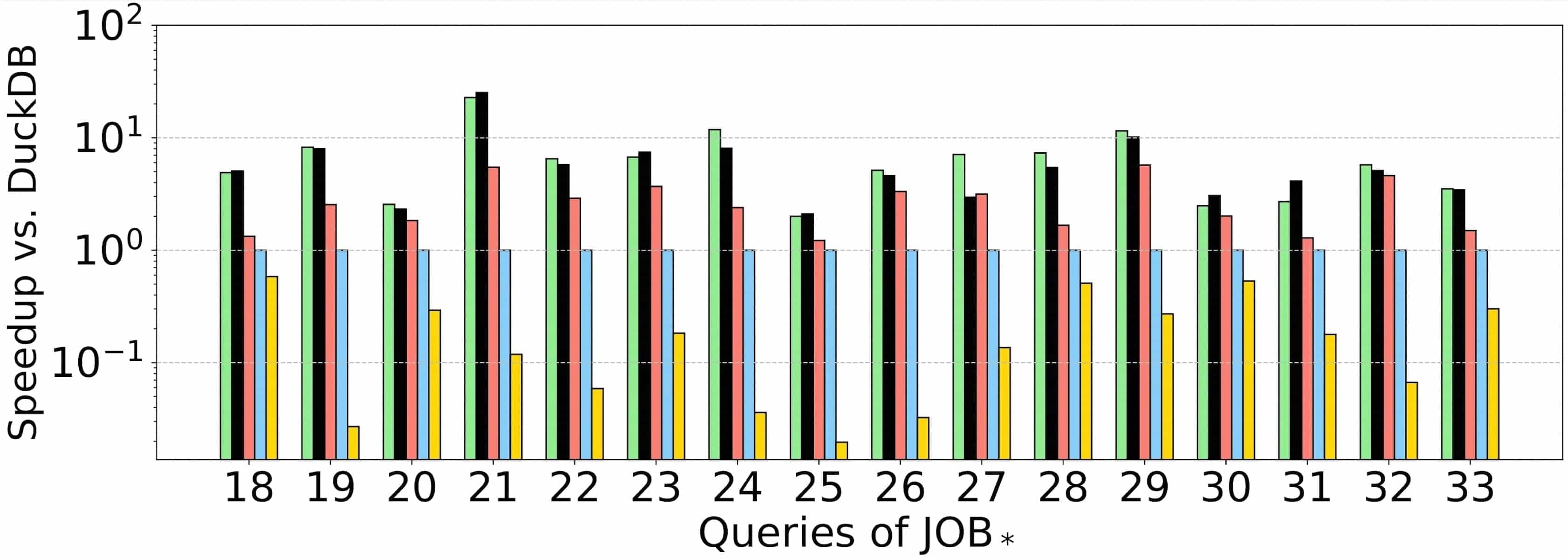 JOB
JOB

Experimental results show that on the LDBC100 dataset, the query plans generated by RelGo have average execution times that are 21.9x, 5.4x, 49.9x, and 188.7x faster than those generated by DuckDB, GRainDB, Umbra, and Kùzu, respectively. This indicates that RelGo has a significant advantage over baseline methods in optimizing graph-related queries.
Another benchmark, i.e., the JOB benchmark that is established for assessing join optimizations in relational databases, lacks any cyclic-pattern queries. On the JOB benchmark, the query plans generated by RelGo have average execution times that are 8.2x, 4.0x, 1.7x, and 136.1x faster than those generated by DuckDB, GRainDB, Umbra, and Kùzu, respectively. This further demonstrates that RelGo can generate more efficient query plans.