Design of GLE
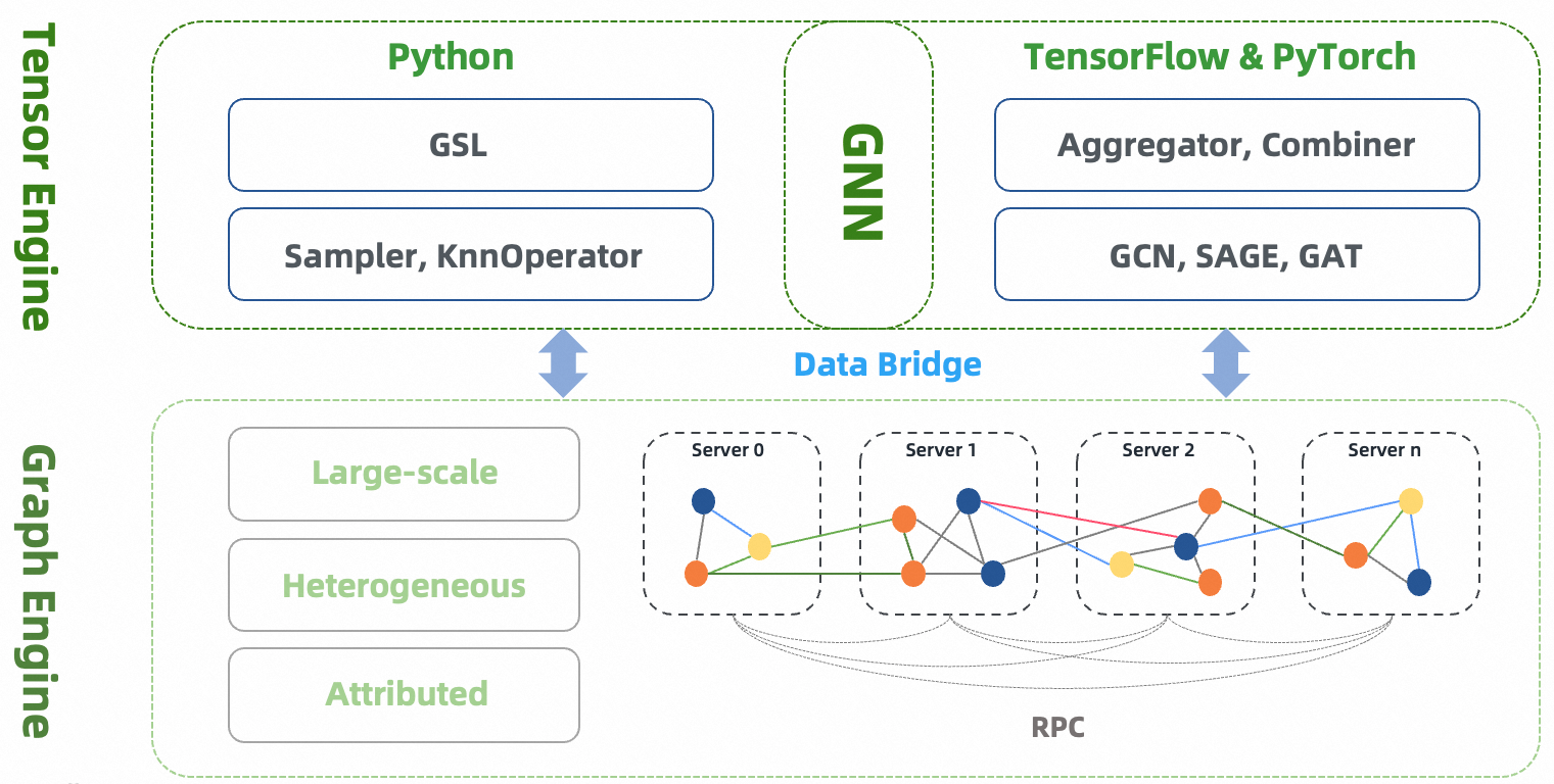
GLE (Graph Learning Engine) is a distributed framework to develop and implement graph neural networks at a large scale. GLE has been successfully applied in various scenarios such as network security, knowledge graph, and search recommendation. It facilitates sampling on batch graphs and enables offline or incremental GNN model training. GLE provides graph sampling operations with both Python and C++ interfaces, and a GSL (Graph Sampling Language) interface that is similar to Gremlin. GLE provides model development paradigms and processes for GNN models, and is compatible with TensorFlow and PyTorch. It offers data layer and model layer interfaces, as well as several model examples.
Model Paradigms
Most GNNs algorithms follow the computational paradigm of message passing or neighbor aggregation, and some frameworks and papers divide the message passing process into aggregate, update, etc. However, in practice, the computational process required by different GNNs algorithms is not exactly the same.
In practical industrial applications, the size of the graph is relatively large and the features on the nodes and edges of the graph are complex (there may be both discrete and continuous features), so it is not possible to perform message passing/neighbor aggregation directly on the original graph. A feasible and efficient approach is based on the idea of sampling, where a subgraph is first sampled from the graph and then computed based on the subgraph. After sampling out the subgraph, the node and edge features of that subgraph are preprocessed and uniformly processed into vectors, and then the computation of efficient message passing can be performed based on that subgraph.
To summarize, we summarize the paradigm of GNNs into 3 stages: subgraph sampling, feature preprocessing, and message passing.
Subgraph sampling: Subgraphs are obtained through GSL sampling provided by GraphLearn, which provides graph data traversal, neighbor sampling, negative sampling, and other functions.
Feature preprocessing: The original features of nodes and edges are preprocessed, such as vectorization (embedding lookup) of discrete features.
Message passing: Aggregation and update of features through topological relations of the graph.
According to the difference of neighbor sampling operator in subgraph sampling and NN operator in message passing, we organize the subgraph into EgoGraph or SubGraph format. EgoGraph consists of central object ego and its fixed-size neighbors, which is a dense organization format. SubGraph is a more general subgraph organization format, consisting of nodes, edges features and edge index (a two-dimensional array consisting of row index and column index of edges), generally using full neighbor. The conv layer based on SubGraph generally uses the sparse NN operator. EgoGraph refers to a subgraph composed of ego (central node) and k-hop neighbors; SubGraph refers to a generalized subgraph represented by nodes, edges and edge_index.
Next, we introduce two different computational paradigms based on EgoGraph and SubGraph.
EgoGraph-based node-centric aggregation
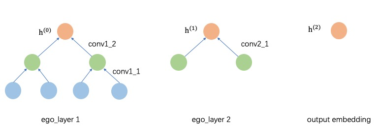
EgoGraph consists of ego and neighbors, and the message aggregation path is determined by the potential relationship between ego and neighbors. k-hop neighbors only need to aggregate the messages of k+1-hop neighbors, and the whole message passing process is carried out along the directed meta-path from neighbors to themselves. In this approach, the number of sampled neighbor hops and the number of layers of the neural network need to be exactly the same. The following figure illustrates the computation of a 2-hop neighbor model of GNNs. The vector of original nodes is noted as h(0); the first layer forward process needs to aggregate 2-hop neighbors to 1-hop neighbors and 1-hop neighbors to itself, the types of different hop neighbors may be different, so the first layer needs two different conv layers (for homogeneous graphs, these two conv layers are the same), and the features of nodes after the first layer are updated to h(1) as the input of the second layer; at the second layer, it needs to aggregate the h(1) of 1-hop neighbors to update the ego node features, and the final output node features h(2) as the embedding of the final output ego node.
SubGraph-based graph message passing
Unlike EgoGraph, SubGraph contains the edge_index of the graph topology, so the message passing path (forward computation path) can be determined directly by the edge_index, and the implementation of the conv layer can be done directly by the edge_index and the nodes/edges data. In addition, SubGraph is fully compatible with the Data in PyG, so the model part of PyG can be reused.
Pipeline for Learning
A GNN training/prediction task usually consists of the following steps.
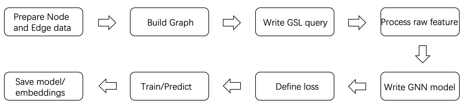
The first step in using GraphLearn is to prepare the graph data according to the application scenario. Graph data exists in the form of a vertex table and an edge table, and an application scenario will usually involve multiple types of vertices and edges. These can be added one by one using the interface provided by GraphLearn. The construction of graph data is a critical part of the process as it determines the upper limit of algorithm learning. It is important to generate reasonable edge data and choose appropriate features that are consistent with business goals.
Once the graph is constructed, samples need to be sampled from the graph to obtain the training samples. It is recommended to use GraphLearn Sample Language (GSL) to construct the sample query. GSL can use GraphLearn’s asynchronous and multi-threaded cache sampling query function to efficiently generate the training sample stream.
The output of GSL is in Numpy format, while the model based on TensorFlow or PyTorch needs data in tensor format. Therefore, the data format needs to be converted first. Additionally, the features of the original graph data may be complex and cannot be directly accessed for model training. For example, node features such as “id=123456, age= 28, city=Beijing” and other plaintexts need to be processed into continuous features by embedding lookup. GraphLearn provides a convenient interface to convert raw data into vector format, and it is important to describe clearly the type, value space, and dimension of each feature after vectorization when adding vertex or edge data sources.
In terms of GNN model construction, GraphLearn encapsulates EgoGraph based layers and models, and SubGraph based layers and models. These can be used to build a GNNs model after selecting a model paradigm that suits your needs. The GNNs model takes EgoGraph or BatchGraph (SubGraph of mini-batch) as input and outputs the embedding of the nodes.
After getting the embedding of the vertices, the loss function is designed with the scenario in mind. Common scenarios can be classified into two categories: node classification and link prediction. For link prediction, the input required includes “embedding of source vertex, embedding of destination vertex, embedding of target vertex with negative sampling”, and the output is the loss. This loss is then optimized by iterating through the trainer. GraphLearn encapsulates some common loss functions that can be found in the section “Common Losses”.